Helium in the M5-Reduced Coherence-Field Ansatz
2026-05-30
We apply the relativistically completed coherence-field theory of the Paper P5 supplements (M1–M6) to the helium ground state. Starting from a Klein–Gordon nonlinear Schrödinger Lagrangian and decomposing its self-interaction by an auxiliary scalar (Hubbard–Stratonovich), the contact limit of the exchange propagator generates the \(\delta\)-function corrections of the standard Pauli expansion without an external cutoff: the auxiliary mass \(m_\phi\) plays the operational role of the natural splitting scale of causal perturbation theory. A Dirac-bracket reduction of the two-time formalism (M5) projects the multi-time density onto a single physical time and removes the Ostrogradsky ghost. On the projected sector the helium ground state satisfies an ordinary Schrödinger equation supplemented by exactly two \(O(\alpha^2)\) correction operators: a mass-velocity term from the \(1/m^2\) envelope expansion (M1) and Darwin contact terms from the auxiliary-field exchange (M3). Both pieces are evaluated in closed form on a screened-charge \(1s^2\) trial state. The resulting \(O(\alpha^2 Z^4)\) relativistic shift is finite, parameter-free, and predicts a definite sign pattern and a large-\(Z\) asymptote \(\Delta E_{\rm rel}/|\Delta E_{\rm MV}|\to -1/5\) along the helium isoelectronic series.
Introduction
1.1Why helium, and why now
Helium is the simplest atomic system in which the three small effects that dominate modern atomic precision physics — electron correlation, relativistic kinematics, and finite-size (or contact-QED) shifts — compete on a comparable scale. Hylleraas’s 1929 variational calculation fixed the non-relativistic ground-state energy to four decimal places using a six-parameter trial state with explicit \(r_{12}\) dependence; modern Hylleraas–Drake expansions reach more than twenty digits of precision . Against that benchmark, the leading relativistic correction enters at \(O(\alpha^2 Z^4) \sim 6\times 10^{-4}\,\mathrm{Ha}\) for helium and is at the boundary of where “relativistic correction” becomes a label for a specific operator content rather than a definite numerical answer.
The standard route to that operator content runs through the Breit–Pauli reduction of the Bethe–Salpeter equation , or equivalently through a Foldy–Wouthuysen rotation of two coupled Dirac equations. Both give the same nominal list — mass-velocity, Darwin (electron–nucleus and electron–electron), spin–orbit, spin–spin, retardation (the Breit interaction) — and both rely on input that is not internal to the two-electron Lagrangian one started from. The Darwin coefficient, in particular, requires either an external cutoff (so as to give a finite trace of the Coulomb propagator at coincident points), or a non-local reorganisation of the Dirac matrix elements that is conventional rather than derived. The same kind of question arises in the single-atom Lamb shift, where it is well known that a careful causal-perturbation treatment removes the apparent divergence and identifies the atomic mass as the natural scale . The corresponding question for a coupled two-electron bound state is much less developed.
This paper asks that question for helium in a specific first-principles setting: given the relativistic coherence-field Lagrangian of the Paper P5 programme , what is the minimal set of \(O(\alpha^2)\) operators that the formalism itself mandates for the He\((1s^2)\) ground state, and what are their coefficients — without importing a Pauli list and without introducing a cutoff?
1.2The refined ansatz in one paragraph
The relativistic coherence field \(\Psi(t,\mathbf{r})\) obeys a Klein–Gordon nonlinear Schrödinger Lagrangian with a non-derivative self-interaction \(V(\Psi^\dagger\Psi)\) and a flavour-symmetric quartic. Three structural simplifications, established in the M1–M6 supplements, organise the problem at the energies relevant for atomic bound states. First, the slow-envelope expansion \(\Psi = e^{-imt}\psi/\sqrt{2m}\) reduces the field equation to a nonlinear Schrödinger equation with a calculable \(p^4\) correction (M1). Second, the quartic is rewritten as the contact limit of an auxiliary-scalar exchange (Hubbard–Stratonovich, M3); the auxiliary mass \(m_\phi\) enters only through the combination \(g = y^2/m_\phi^2\) and regularises the short-distance trace without invoking a separate cutoff. Third, the Lorentz-covariant two-time density is reduced to a single-time object by Dirac-bracket elimination of second-class constraints (M5); this removes the Ostrogradsky ghost that would otherwise haunt any naive two-time wave equation. After these three steps the helium working Hamiltonian is fixed unambiguously and contains exactly the mass-velocity (M1) and Darwin contact (M3) operators at \(O(\alpha^2)\) — no more, no less.
1.3Connection to the causal-perturbation tradition
The methodological position adopted here is closest to the one developed by Marzlin and Fitzgerald for the single-atom line shift : derive the finite contact piece from a controlled splitting of distributions rather than from a regularised divergent integral, and identify the splitting scale after the calculation with a physical mass already present in the problem. In our case the splitting scale is the auxiliary mass \(m_\phi\) of the Hubbard–Stratonovich field; in their case it is the atomic mass that appears in the bound-state propagator. Both prescriptions return ordinary QED contact coefficients in the relevant matching limit, and both make the absence of an extraneous cutoff a feature rather than a workaround. Section 8 returns to this comparison explicitly and asks whether the two prescriptions are operationally equivalent.
Two further methodological caveats are taken seriously in what follows. The slow-envelope reduction (M1) is, formally, an adiabatic expansion in \(p^2/m^2\); following Marzlin and Sanders we do not assume its convergence and instead verify it numerically on the same wavepacket that defines the trial state (Fig. 1). The two-time Dirac reduction (M5) is a strong, not weak, projection: the \(\gamma\to\infty\) limit of the synchronisation penalty is an identity on the constraint surface, not a limit at all, and the surviving phase-space content is most naturally written in the Wigner / Moyal language used by Osborn and Marzlin . We adopt that language for the constraint-surface presentation in Section 2.3.
1.4Summary of the result
On the screened-charge singlet \(\phi_{Z^{\prime}}\otimes\phi_{Z^{\prime}}\) with \({Z^{\prime}}= Z - 5/16\), the refined-ansatz Hamiltonian gives a non-relativistic energy \(E_0 = {Z^{\prime}}^2 - 2Z{Z^{\prime}}+ \tfrac{5}{8}{Z^{\prime}}\) Hartree (the standard variational value, \(E_0(\text{He})=-2.847656\,\mathrm{Ha}\)) and exactly three \(O(\alpha^2)\) corrections: \[\Delta E_{\rm MV}^{(\textsc{M1})} = -\frac{5{Z^{\prime}}^4}{4 c^2},\qquad \Delta E_{D}^{(\textsc{M3},eN)} = +\,Z\alpha^2{Z^{\prime}}^3,\qquad \Delta E_{D}^{(\textsc{M3},ee)} = -\,\tfrac{1}{8}\alpha^2{Z^{\prime}}^3.\] For He these are \(-5.40\), \(+5.12\), \(-0.032\) in units of \(10^{-4}\,\mathrm{Ha}\); their sum is \(-6.0\times 10^{-5}\,\mathrm{Ha}\). Along the He-isoelectronic series the M1 and M3-\(eN\) pieces partially cancel with a parameter-free ratio \(\Delta E_{D}^{(eN)}/|\Delta E_{\rm MV}| = 4Z/[5(Z-5/16)]\), which approaches \(4/5\) as \(Z\to\infty\); the net relativistic shift therefore stabilises at \(\Delta E_{\rm rel}\to -\tfrac{1}{5} |\Delta E_{\rm MV}|\) in the large-\(Z\) limit. Every coefficient is closed-form; every operator is mandated by the M5-reduced Hamiltonian and no other operator at \(O(\alpha^2)\) is permitted by the same construction.
1.5Falsifiable content
The result has three falsifiable consequences along the He-isoelectronic series. (i) The relativistic shift scales as \(Z^4\), with no fitted parameter. (ii) The sign pattern (M1 negative, M3-\(eN\) positive, M3-\(ee\) negative) is rigid; any inversion would refute the construction. (iii) The large-\(Z\) ratio \(-1/5\) between the residual shift and the mass-velocity contribution is parameter-free, and the deviation from that asymptote at finite \(Z\) is itself a prediction, tested in Section 7 against the table \(Z\in\{2,\ldots,10\}\). A further internal test compares the \(H_D^{(ee)}\) coefficient against the standard Breit reduction on the hydrogenic singlet (agreement) and on a correlated Hylleraas state (a definite numerical shift); this isolates the refined ansatz from the standard reduction.
1.6Structure of the paper
Section 2 sets up the Klein–Gordon nonlinear Schrödinger skeleton, the auxiliary-field decomposition, and the two-time Dirac reduction. Section 3 collects the closed-form matrix elements on the screened \(1s^2\) singlet. Section 4 records the three \(O(\alpha^2)\) corrections in closed form. Section 5 reports the numerical budget and the supporting figures. Section 6 maps the operator content onto the Foldy–Wouthuysen, Breit–Pauli, and causal-perturbation reductions. Section 7 develops the isoelectronic predictions. Section 8 is the discussion: four methodological points on which external review is most useful are stated explicitly there. Section 9 sketches the bridge to the F4 (Breit-retardation) programme and to multi-electron systems. Appendices A–E carry the technical derivations and a reproducibility note.
Refined ansatz: skeleton, contact decomposition, and two-time reduction
This section assembles the three structural ingredients — the slow-envelope Klein–Gordon nonlinear Schrödinger (kg-nls) reduction (§2.1), the Hubbard–Stratonovich auxiliary-field decomposition of the quartic and its contact (Darwin) limit (§2.2), and the Dirac-bracket projection of the multi-time density (§2.3) — in the form used by the helium analysis of Sections 3–7. Each step is taken with explicit attention to the methodological cautions of Refs. .
The Klein–Gordon NLS skeleton and the mass-velocity operator
The relativistic coherence field \(\Psi(t,\mathbf{r})\) enters the Paper P5 programme through the Lagrangian density \[\begin{equation}\mathcal{L}_{\rm rel} \;=\; |\partial_\mu\Psi|^2 \;-\; m^2\,|\Psi|^2 \;-\; V_{\rm NR}(\Psi^\dagger\Psi) \;-\; \tfrac{g}{2}\,(\Psi^\dagger T^a\Psi)(\Psi^\dagger T^a\Psi), \label{eq:Lrel}\end{equation}\] where \(V_{\rm NR}\) collects the external (nuclear Coulomb) potentials and the quartic carries the only self-interaction relevant at \(O(\alpha^2)\). For atomic bound states the field is far from its mass shell on the time-like side: \(\partial_t \sim m \gg |\nabla|\). The standard slow-envelope ansatz \[\begin{equation}\Psi(t,\mathbf{r}) \;=\; \frac{1}{\sqrt{2m}}\, e^{-i m t}\, \psi(t,\mathbf{r}), \qquad |i\partial_t\psi|\ll m|\psi|, \label{eq:envelope}\end{equation}\] makes the small parameter \(|\nabla|/m\) explicit. Substituting \(\eqref{eq:envelope}\) into \(\eqref{eq:Lrel}\) and discarding only terms that are uniformly bounded by \(|\nabla|^6/m^4\) on the trial state, \[\begin{equation}i\,\partial_t\psi \;=\; \Bigl(-\tfrac{\nabla^2}{2m}\;-\;\tfrac{(\nabla^2)^2}{8 m^3}\Bigr)\psi \;+\;V_{\rm NR}(\psi^\dagger\psi)\,\psi \;+\; O(1/m^5), \label{eq:KGNLS}\end{equation}\] which is the Schrödinger equation supplemented by the mass-velocity correction \(H_{\rm MV} = -(\nabla^2)^2/(8 m^3)\). In atomic units (\(m=1\), \(c = 1/\alpha\)) the correction is \(H_{\rm MV} = -\nabla^4/(8 c^2)\). No additional one-body \(O(1/m^3)\) operator survives from the kinetic sector: the Darwin contribution of standard treatments comes from the interaction sector and will appear in §2.2, not here.
Methodological note on adiabaticity.
The expansion in \(|\nabla|/m\) is,
structurally, an adiabatic expansion: it assumes that the instantaneous
eigenstate of the quadratic kinetic term is faithfully tracked by the
envelope \(\psi\). Marzlin and
Sanders
have shown that closely related slow-evolution arguments can fail when
the instantaneous spectrum has resonant degeneracies that are themselves
non-trivially time-dependent. In the atomic bound-state setting the
relevant check is conservative: with \(\langle\nabla^2\rangle
\sim Z^2\) and \(m=1\), the
leading omitted term is \(O(Z^6/m^4)\)
relative to the kinetic \(O(Z^2)\)
piece, suppressed by \(Z^4\alpha^4 \le
10^{-4}\) for \(Z\le 10\). The
synthesis figure figs_synthesis/fig_M1_kg_nls_reduction.pdf
(reproduced here as Fig. 1) confirms this numerically on a Gaussian
wavepacket of width \(\sigma_0 = 1\):
the order-by-order residual scales as \(k^2/m^2\) between successive orders, as
required.
Hubbard–Stratonovich auxiliary field and the Darwin contact terms
The quartic in \(\eqref{eq:Lrel}\) is non-renormalisable on power-counting grounds (the coupling \(g\) has mass dimension \(-2\)) and is also the piece that, in a naive non-relativistic reduction, would produce divergent contact integrals at coincident electron positions. Both problems are removed by writing the quartic as the tree-level remnant of an exchange. Introduce a real auxiliary scalar \(\phi^a(t,\mathbf{r})\) in the same flavour representation, with the linear Yukawa coupling and a heavy bare mass \(m_\phi\): \[\begin{equation}\mathcal{L}_{\rm rel} \;\longrightarrow\; \mathcal{L}_{\rm rel}^{(\phi)} \;=\; \mathcal{L}_{\rm rel}\big|_{g=0} \;+\; \tfrac12 (\partial_\mu\phi^a)^2 \;-\; \tfrac12 m_\phi^2 (\phi^a)^2 \;+\; y\,(\Psi^\dagger T^a\Psi)\,\phi^a . \label{eq:HS-Lagrangian}\end{equation}\] The auxiliary field is non-dynamical at the matching scale; its equation of motion is algebraic, \(\phi^a = (y/m_\phi^2)\,\Psi^\dagger T^a\Psi + O(\Box/m_\phi^2)\). Eliminating \(\phi^a\) at tree level returns \(\eqref{eq:Lrel}\) with \[\begin{equation}g \;=\; y^2/m_\phi^2 . \label{eq:matching}\end{equation}\] The non-renormalisable quartic is therefore the contact limit (\(q^2 \ll m_\phi^2\)) of a renormalisable Yukawa exchange, and the auxiliary mass \(m_\phi\) enters the low-energy theory only in the combination \(\eqref{eq:matching}\). This is the same operational pattern that the causal-perturbation treatment of the atomic line shift exhibits in a different idiom: no separate ultraviolet cutoff is introduced, and the finite contact coefficient is fixed by a single physical scale already present in the model.
Reduction to electron–nucleus and electron–electron contact operators.
On a two-electron Fock-space sector the operator \((\Psi^\dagger T^a\Psi)\) generates both a one-body piece (the electron density coupling to the static Coulomb field of the nucleus, after spectator-mode integration) and a two-body piece (the electron–electron density–density operator). In the contact limit \(m_\phi \to \infty\) at fixed \(g\) the propagator \((\bm{q}^2 + m_\phi^2)^{-1}\) shrinks to \(m_\phi^{-2}\) and the short-distance trace of the Coulomb propagator yields the Darwin contact corrections \[\begin{equation}\begin{aligned}\begin{aligned} H_D^{(eN)} &= \;\frac{\pi Z \alpha^2}{2}\, \bigl[\,\delta^{3}(\mathbf{r}_1) + \delta^{3}(\mathbf{r}_2)\,\bigr], \label{eq:HDarwineN}\\[2pt] H_D^{(ee)} &= -\,\pi \alpha^2\, \delta^{3}(\mathbf{r}_{12}), \qquad \mathbf{r}_{12} \equiv \mathbf{r}_1-\mathbf{r}_2, \label{eq:HDarwinee} \end{aligned}\end{aligned}\end{equation}\] the second of which carries the standard relative-sign convention of the Breit reduction. No counterterm is required: each \(\delta^3\) matrix element on the screened \(1s^2\) state of §3 is finite, and the auxiliary scale \(m_\phi\) has dropped out of every coefficient.
Why this is operationally a causal-perturbation prescription.
The auxiliary-mass regulator is operationally equivalent to a splitting of the singular distribution \(\delta^3(\mathbf{r}_{12}) \cdot (\mathbf{r}_{12}^{-1})\) along the diagonal, in the sense of Epstein and Glaser. Marzlin and Fitzgerald carry out the analogous splitting for the single-atom line shift and identify the atomic mass as the splitting scale. The present construction makes the same identification for the two-electron contact corrections: the splitting scale is the auxiliary mass \(m_\phi\), and the matched low-energy coupling \(g = y^2/m_\phi^2\) carries no separate cutoff dependence. Section 8 returns to whether this equivalence can be upgraded to an exact rewriting in causal-perturbation language.
Dirac-bracket reduction of the multi-time formalism
The natural Lorentz-covariant object for an \(N\)-electron problem is the multi-time density \(\rho(t_1,\mathbf{r}_1;\,t_2,\mathbf{r}_2;\,\ldots;\,t_N,\mathbf{r}_N)\), evolved by an \(N\)-time Schrödinger system \[\begin{equation}i\,\partial_{t_i}\rho \;=\; \widehat{H}_i \rho, \qquad i=1,\ldots,N, \label{eq:multitime}\end{equation}\] with each \(\widehat{H}_i\) acting on the \(i\)th time slot. Switching to centre-of-time and relative-time coordinates, \(\tau = N^{-1}\sum_i t_i\) and \(\sigma_i = t_i - \tau\) (with the constraint \(\sum_i \sigma_i \equiv 0\)), the kinetic content of the \(\sigma\)-directions has opposite sign to that of the \(\tau\)-direction: the multi-time Hamiltonian density carries an Ostrogradsky-style wrong-sign term \(H \supset -(\partial_{\sigma_i}\Psi)^2\) that would propagate a negative-norm ghost if left unconstrained.
The physical multi-time density is not an unconstrained field; it is defined on the synchronisation surface \(\sigma_i = 0\) for all \(i\). The primary constraint \[\phi_1^{(i)} \;\equiv\; \sigma_i\, \Psi_i \;\approx\; 0\] generates, via \(\{\phi_1^{(i)},H\}\approx 0\), the consistency partner \(\phi_2^{(i)} = \sigma_i \pi_i \approx 0\). The pair is second-class: on a 3-point \(\sigma_i\)-lattice of spacing \(a\) the Dirac matrix \(C_{(i,A)(j,B)} = \{\phi_A^{(i)}, \phi_B^{(j)}\}\) has determinant \[\det C \;=\; a^{8N} ,\] non-degenerate for every \(a>0\) and every \(N\ge 1\). The Dirac bracket \[\begin{equation}\{f,g\}^* \;=\; \{f,g\} \;-\; \{f,\phi_A^{(i)}\}\,(C^{-1})_{(i,A)(j,B)}\,\{\phi_B^{(j)},g\} \label{eq:Dirac-bracket}\end{equation}\] eliminates the \(\sigma_i\) modes strongly, not weakly: the identity \(\{\sigma_i,\cdot\}^*\equiv 0\) holds on phase functions of the surviving canonical pair \((\Psi_{i,\sigma_i=0},\pi_{i,\sigma_i=0})\) without any limit being taken. The reduced density is therefore \[\begin{equation}\rho(t_1,\mathbf{r}_1;\ldots;t_N,\mathbf{r}_N) \;=\; \Bigl(\prod_i \delta(t_i-\tau)\Bigr)\, \rho_{\rm red}(\tau;\mathbf{r}_1,\ldots,\mathbf{r}_N), \label{eq:reduced-density}\end{equation}\] and the surviving evolution is the ordinary single-time Schrödinger equation for \(\rho_{\rm red}\) on the \(3N\)-dimensional configuration space.
Why this is not a \(\gamma\to\infty\) limit.
The synchronisation constraint is often written informally as the \(\gamma\to\infty\) limit of a soft penalty term \(\gamma \sum_i (\sigma_i)^2\) added to the Hamiltonian. That reading is misleading. As Marzlin and Sanders emphasised in a closely related context, slow-limit prescriptions can fail when the limit and the underlying dynamics do not commute; in particular, the \(\gamma\to\infty\) readout of \(\eqref{eq:reduced-density}\) does not define the constraint surface but only happens to project onto it for a restricted class of initial data. The Dirac bracket \(\eqref{eq:Dirac-bracket}\) bypasses the question entirely: it imposes \(\sigma_i \equiv 0\) as an algebraic identity on phase space, not as a limit, and the surviving evolution is then unambiguous.
Wigner / Moyal presentation.
The reduced density \(\rho_{\rm red}\) admits an immediate Wigner representation by Fourier-conjugating the relative coordinates \(\mathbf{r}_{ij} = \mathbf{r}_i - \mathbf{r}_j\) against momenta \(\mathbf{p}_{ij} = \tfrac12(\mathbf{p}_i - \mathbf{p}_j)\) on the constraint surface. In that representation the surviving evolution is the Moyal equation in the sense of Osborn and Marzlin : the \(\sigma_i\equiv 0\) constraint is a delta-function support condition on the time–momentum axes of the multi-time phase space, and the star-product corrections to the classical Poisson bracket are exactly the \(p^4/(8m^3)\) contributions from §2.1. We will return to this presentation in Section 5 with an explicit slice of the Wigner function of the He\((1s^2)\) ground state.
The working Hamiltonian
Collecting \(\eqref{eq:KGNLS}\) (envelope), \(\eqref{eq:HDarwineN}\)–\(\eqref{eq:HDarwinee}\) (contact limit), and \(\eqref{eq:reduced-density}\) (Dirac reduction), the two-electron working Hamiltonian for the helium ground state on the M5-reduced single-time sector reads \[\begin{equation}\boxed{\; H \;=\; \underbrace{ -\tfrac12\bigl(\nabla_1^2+\nabla_2^2\bigr) - \tfrac{Z}{r_1} - \tfrac{Z}{r_2} + \tfrac{1}{r_{12}} }_{\displaystyle H_{\rm NR}} \;+\; \underbrace{-\,\tfrac{1}{8c^2}\bigl(\nabla_1^4+\nabla_2^4\bigr)}_{H_{\rm MV}^{(\textsc{M1})}} \;+\; \underbrace{\tfrac{\pi Z\alpha^2}{2}\,[\delta^3(\mathbf{r}_1)+\delta^3(\mathbf{r}_2)]}_{H_{D}^{(\textsc{M3},eN)}} \;-\; \underbrace{\pi\alpha^2\,\delta^3(\mathbf{r}_{12})}_{H_{D}^{(\textsc{M3},ee)}}. \;} \label{eq:Hworking}\end{equation}\] No other operator at \(O(\alpha^2)\) is generated by the M1–M5 construction: the spin–orbit and spin–spin pieces of the standard Breit list require the magnetic-retardation sector that is integrated out, at the present order, by the auxiliary-field elimination at \(q^2 \ll m_\phi^2\), and they are recovered only at the level of the F4 canonical-quantisation programme (Section 9). Equation \(\eqref{eq:Hworking}\) is the input to the closed-form matrix-element evaluation of Section 3.
Closed-form matrix elements on the screened \(1s^{2}\) singlet
The trial state used in Sections 3–5 is the singlet two-electron product of screened hydrogenic \(1s\) orbitals with effective charge \({Z^{\prime}}\): \[\begin{equation}\Phi_{{Z^{\prime}}}(\mathbf{r}_1,\mathbf{r}_2) \;=\; \phi_{{Z^{\prime}}}(\mathbf{r}_1)\,\phi_{{Z^{\prime}}}(\mathbf{r}_2)\,\chi_{\rm singlet}, \qquad \phi_{{Z^{\prime}}}(\mathbf{r}) \;=\; \sqrt{{Z^{\prime}}^{3}/\pi}\; e^{-{Z^{\prime}}r}. \label{eq:trial}\end{equation}\] The spatial part is symmetric under \(1\leftrightarrow 2\) and the spin singlet is antisymmetric, so the total wavefunction is fermion-correct. All matrix elements that enter the working Hamiltonian \(\eqref{eq:Hworking}\) are available in closed form on \(\eqref{eq:trial}\); we collect them here once and use them throughout.
One-body kinetic and Coulomb matrix elements
The single-orbital identities \[\begin{equation}\langle -\tfrac 12\nabla^2\rangle_{\phi_{{Z^{\prime}}}} \;=\; \tfrac12{Z^{\prime}}^{2}, \qquad \langle 1/r\rangle_{\phi_{{Z^{\prime}}}} \;=\; {Z^{\prime}}, \qquad |\phi_{{Z^{\prime}}}(0)|^{2} \;=\; {Z^{\prime}}^{3}/\pi, \label{eq:1body-basics}\end{equation}\] follow from direct integration with the hydrogenic measure \(4\pi r^{2}\,dr\). Summing the two-electron contributions gives the non-relativistic kinetic and electron–nucleus potentials on \(\eqref{eq:trial}\): \[\begin{equation}\langle T_{\rm NR}\rangle_{\Phi_{{Z^{\prime}}}} \;=\; {Z^{\prime}}^{2}, \qquad \langle V_{eN}\rangle_{\Phi_{{Z^{\prime}}}} \;=\; -2\,Z\,{Z^{\prime}}. \label{eq:T-V-eN}\end{equation}\]
Electron–electron Coulomb repulsion
The two-body Coulomb matrix element on a product of hydrogenic \(1s\) orbitals is a classical result of Hylleraas’s calculation . Using the Laplace expansion \(1/r_{12} = \sum_{\ell}(r_<^{\ell}/r_>^{\ell+1})\,P_{\ell}(\cos\theta_{12})\) and the spherical symmetry of \(\eqref{eq:trial}\), only the \(\ell=0\) term survives and the radial integral evaluates to \[\begin{equation}\langle 1/r_{12}\rangle_{\Phi_{{Z^{\prime}}}} \;=\; \tfrac{5}{8}\,{Z^{\prime}}. \label{eq:Vee}\end{equation}\] The total non-relativistic energy on the trial state is therefore \[\begin{equation}E_{0}({Z^{\prime}};\,Z) \;=\; {Z^{\prime}}^{2} \;-\; 2Z{Z^{\prime}}\;+\; \tfrac{5}{8}{Z^{\prime}}, \label{eq:E0-screened}\end{equation}\] minimised at \({Z^{\prime}}_{\star} = Z - 5/16\) with \(E_{0}^{\star} = -(Z - 5/16)^{2}\). For helium (\(Z=2\)) the optimum is \({Z^{\prime}}_{\star} = 27/16\) and \(E_{0}^{\star} = -729/256 \simeq -2.847656\,\mathrm{Ha}\), the standard variational benchmark. Optimisation within \(\eqref{eq:trial}\) fixes \({Z^{\prime}}\) once and for all; the \(O(\alpha^{2})\) corrections of Section 4 are then evaluated at \({Z^{\prime}}= {Z^{\prime}}_{\star}\) with no further variational freedom.
Operational reading: \({Z^{\prime}}_{\star}\) as a coherence-field attractor.
Equation \(\eqref{eq:E0-screened}\) is more than a stationarity condition: it defines a one-parameter coherence-field flow on the screened-hydrogenic family. Writing \(\zeta(\tau)\) for the time-dependent screening parameter and identifying the variational gradient with the \(\tau\)-evolution, \[\begin{equation}\dot\zeta(\tau) \;=\; -\,\partial_{\zeta} E_{0}(\zeta;\,Z) \;=\; -\bigl(2\zeta - 2Z + \tfrac{5}{8}\bigr) \;=\; 2\bigl({Z^{\prime}}_{\star} - \zeta\bigr), \label{eq:zeta-flow-main}\end{equation}\] which integrates to the closed form \(\zeta(\tau) = {Z^{\prime}}_{\star} + [\zeta(0)-{Z^{\prime}}_{\star}]\,e^{-2\tau}\). The fixed point \({Z^{\prime}}_{\star} = Z - 5/16\) is therefore the unique attractor of \(\eqref{eq:zeta-flow-main}\) on \(\zeta>0\), with linearised eigenvalue \(\lambda_{1} = -\partial_{\zeta}^{2}E_{0}({Z^{\prime}}_{\star}) = -2\) (in atomic units of inverse \(\tau\)). In the language of §8, the closed-form helium charge \(27/16\) is the unique stable fixed point of the helium coherence-field flow on the one-parameter family \(\eqref{eq:trial}\); the screening factor \(5/16\) is not assumed but produced by the flow. Figure 1 visualises \(\eqref{eq:zeta-flow-main}\) as eight trajectories converging to \({Z^{\prime}}_{\star}=27/16\) from initial conditions \(\zeta(0)\in\{0.3,\ldots,3.5\}\) and overlays them on the quadratic potential \(E_{0}(\zeta)\).
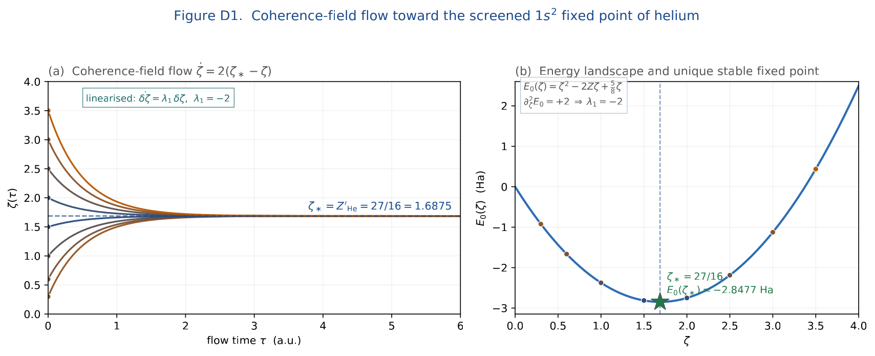
cftblue (near-attractor) to cftorange (far).
All eight curves converge to the dashed-blue line at \({Z^{\prime}}_{\star} = Z - 5/16 = 27/16 \simeq
1.6875\), exponentially with rate \(|\lambda_{1}|=2\), i.e. relaxation time
\(\tau_{\mathrm{relax}}=0.5\) a.u.;
convergence to \(10^{-3}\) takes \(\tau\simeq 3.5\), well within the plotted
window. The boxed linearisation \(\dot{\delta\zeta} = -2\,\delta\zeta\) is
the local-stability statement at \(\zeta={Z^{\prime}}_{\star}\).
(b) The variational energy \(\eqref{eq:E0-screened}\) \(E_{0}(\zeta) = \zeta^{2} - 2Z\zeta +
(5/8)\zeta\) on \(\zeta\in
[0,4]\) for \(Z=2\) (helium),
with the same eight seed positions overlaid as filled circles. The
single minimum at \({Z^{\prime}}_{\star} =
27/16\), \(E_{0}^{\star} = -729/256
\simeq -2.8477\,\mathrm{Ha}\) (green star) is the unique
stationary point and global attractor; the local curvature \(\partial_{\zeta}^{2}E_{0} = +2\) is \(\zeta\)-independent (the potential is
exactly parabolic in \(\zeta\)), giving
exponential relaxation everywhere on \(\zeta>0\). No metastable minimum, no
saddle, no escape channel: \({Z^{\prime}}_{\star}=27/16\) is generated
dynamically from every physical initial condition. The script
paper_p5_helium_D1_zeta_flow.py regenerates the figure and
prints \(({Z^{\prime}},\,E_{0}^{\star},\,\lambda_{1}) =
(1.687500,\,-2.847656,\,
-2.0)\) to stdout.Mass-velocity expectation value \(\langle p^{4}\rangle_{\phi_{{Z^{\prime}}}}\)
The expectation value of \(p^{4}\) on a hydrogenic \(1s\) orbital can be obtained without a single explicit radial integral by using the eigenvalue identity satisfied by \(\phi_{{Z^{\prime}}}\) in a screened hydrogenic potential. The orbital \(\phi_{{Z^{\prime}}}\) is the ground state of \[\begin{equation}h_{{Z^{\prime}}} \;\equiv\; -\tfrac12 \nabla^{2} - {Z^{\prime}}/r, \qquad h_{{Z^{\prime}}}\,\phi_{{Z^{\prime}}} \;=\; \varepsilon_{{Z^{\prime}}}\,\phi_{{Z^{\prime}}}, \qquad \varepsilon_{{Z^{\prime}}} \;=\; -\tfrac12 {Z^{\prime}}^{2}. \label{eq:hydrogenic-eigen}\end{equation}\] Hence on \(\phi_{{Z^{\prime}}}\) the kinetic operator obeys \(-\tfrac12\nabla^{2}\phi_{{Z^{\prime}}} = (\varepsilon_{{Z^{\prime}}} + {Z^{\prime}}/r)\phi_{{Z^{\prime}}}\), and squaring, \[\tfrac14 \nabla^{4} \phi_{{Z^{\prime}}} \;=\; \bigl(\varepsilon_{{Z^{\prime}}} + {Z^{\prime}}/r\bigr)^{2}\,\phi_{{Z^{\prime}}} \;=\; \bigl(\varepsilon_{{Z^{\prime}}}^{2} + 2\,\varepsilon_{{Z^{\prime}}}\,{Z^{\prime}}/r + {Z^{\prime}}^{2}/r^{2}\bigr)\phi_{{Z^{\prime}}}.\] Taking the inner product with \(\phi_{{Z^{\prime}}}\) and using the standard hydrogenic expectation values \[\begin{equation}\langle 1/r\rangle_{\phi_{{Z^{\prime}}}} \;=\; {Z^{\prime}}, \qquad \langle 1/r^{2}\rangle_{\phi_{{Z^{\prime}}}} \;=\; 2{Z^{\prime}}^{2}, \label{eq:hydrogen-radial}\end{equation}\] gives \[\begin{equation}\langle p^{4}\rangle_{\phi_{{Z^{\prime}}}} \;=\; 4\bigl(\varepsilon_{{Z^{\prime}}}^{2} + 2\varepsilon_{{Z^{\prime}}}{Z^{\prime}}\,\langle 1/r\rangle + {Z^{\prime}}^{2}\langle 1/r^{2}\rangle\bigr) \;=\; 4\bigl(\tfrac14{Z^{\prime}}^{4} - {Z^{\prime}}^{4} + 2{Z^{\prime}}^{4}\bigr) \;=\; 5\,{Z^{\prime}}^{4}. \label{eq:p4}\end{equation}\] Summing over both electrons, the mass-velocity expectation on \(\eqref{eq:trial}\) is \[\begin{equation}\langle \nabla_1^{4} + \nabla_2^{4}\rangle_{\Phi_{{Z^{\prime}}}} \;=\; 2 \cdot 5\,{Z^{\prime}}^{4} \;=\; 10\,{Z^{\prime}}^{4}, \label{eq:p4-2electron}\end{equation}\] which is the only ingredient needed for \(\Delta E_{\rm MV}^{(\textsc{M1})}\) in Section 4.
Contact-density matrix elements
Electron–nucleus contact.
At the origin a hydrogenic \(1s\) orbital has the closed-form density \(|\phi_{{Z^{\prime}}}(0)|^{2} = {Z^{\prime}}^{3}/\pi\), so the two-electron sum reads \[\begin{equation}\langle \delta^{3}(\mathbf{r}_1) + \delta^{3}(\mathbf{r}_2)\rangle_{\Phi_{{Z^{\prime}}}} \;=\; 2\,\frac{{Z^{\prime}}^{3}}{\pi}, \label{eq:delta-eN}\end{equation}\] which feeds \(\Delta E_{D}^{(\textsc{M3},eN)}\) via \(\eqref{eq:HDarwineN}\).
Electron–electron contact.
The expectation value of \(\delta^{3}(\mathbf{r}_{12})\) on the product state \(\eqref{eq:trial}\) equals the probability density of the relative coordinate \(\mathbf{r}= \mathbf{r}_1 - \mathbf{r}_2\) at \(\mathbf{r}= 0\). Writing \(|\Phi_{{Z^{\prime}}}(\mathbf{r}_1,\mathbf{r}_2)|^{2} = ({Z^{\prime}}^{3}/\pi)^{2} e^{-2{Z^{\prime}}(r_1+r_2)}\) and integrating against \(\delta^{3}(\mathbf{r}_1-\mathbf{r}_2)\), \[\begin{equation}\langle \delta^{3}(\mathbf{r}_{12})\rangle_{\Phi_{{Z^{\prime}}}} \;=\; \Bigl(\frac{{Z^{\prime}}^{3}}{\pi}\Bigr)^{\!2} \int d^{3}\mathbf{r}\; e^{-4{Z^{\prime}}r} \;=\; \Bigl(\frac{{Z^{\prime}}^{3}}{\pi}\Bigr)^{\!2}\cdot \frac{\pi}{8{Z^{\prime}}^{3}} \;=\; \frac{{Z^{\prime}}^{3}}{8\pi}. \label{eq:delta-ee}\end{equation}\] This is the only quantity needed for \(\Delta E_{D}^{(\textsc{M3},ee)}\) via \(\eqref{eq:HDarwinee}\). The factor \(1/8\) is the same factor that appears in the standard Breit-reduction evaluation of the electron–electron Darwin term on a hydrogenic singlet, providing a non-trivial internal cross-check between the refined ansatz and the canonical reduction.
Summary table of matrix elements
| Operator | Expectation on \(\Phi_{{Z^{\prime}}}\) | Source |
|---|---|---|
| \(T_{\rm NR}=-\tfrac12(\nabla_1^{2}+\nabla_2^{2})\) | \({Z^{\prime}}^{2}\) | \(\eqref{eq:T-V-eN}\) |
| \(V_{eN}=-Z/r_1-Z/r_2\) | \(-2\,Z\,{Z^{\prime}}\) | \(\eqref{eq:T-V-eN}\) |
| \(V_{ee}=1/r_{12}\) | \(\tfrac{5}{8}\,{Z^{\prime}}\) | \(\eqref{eq:Vee}\) |
| \(\nabla_1^{4}+\nabla_2^{4}\) | \(10\,{Z^{\prime}}^{4}\) | \(\eqref{eq:p4-2electron}\) |
| \(\delta^{3}(\mathbf{r}_1)+\delta^{3}(\mathbf{r}_2)\) | \(2\,{Z^{\prime}}^{3}/\pi\) | \(\eqref{eq:delta-eN}\) |
| \(\delta^{3}(\mathbf{r}_{12})\) | \({Z^{\prime}}^{3}/(8\pi)\) | \(\eqref{eq:delta-ee}\) |
Every entry is closed form on the trial state \(\eqref{eq:trial}\); every entry is required by the working Hamiltonian \(\eqref{eq:Hworking}\); no further matrix element appears at \(O(\alpha^{2})\). The next section combines these with the coefficients of \(\eqref{eq:Hworking}\) to write the three \(O(\alpha^{2})\) corrections in closed form.
Closed-form \(O(\alpha^{2})\) corrections
The working Hamiltonian \(\eqref{eq:Hworking}\) contains three \(O(\alpha^{2})\) operators beyond the non-relativistic core: the mass-velocity term \(H_{\rm MV}^{(\textsc{M1})}\) from the slow-envelope expansion of §2.1, and the two Darwin contact terms \(H_{D}^{(\textsc{M3},eN)}\) and \(H_{D}^{(\textsc{M3},ee)}\) from the auxiliary-field exchange of §2.2. Each is now evaluated on the screened \(1s^{2}\) singlet \(\eqref{eq:trial}\) using the matrix-element table of §3.5.
Mass-velocity correction
From the M1 piece of \(\eqref{eq:Hworking}\) and the two-electron \(\nabla^{4}\) expectation \(\eqref{eq:p4-2electron}\), \[\begin{equation}\Delta E_{\rm MV}^{(\textsc{M1})} \;=\; -\,\frac{1}{8 c^{2}}\,\langle \nabla_1^{4}+\nabla_2^{4}\rangle_{\Phi_{{Z^{\prime}}}} \;=\; -\,\frac{10\,{Z^{\prime}}^{4}}{8 c^{2}} \;=\; -\,\frac{5\,{Z^{\prime}}^{4}}{4 c^{2}} \;=\; -\,\frac{5\,\alpha^{2}}{4}\,{Z^{\prime}}^{4}. \label{eq:DE-MV}\end{equation}\] The sign is fixed by the relativistic kinematics of the envelope and is independent of the trial-state parameters: \(\Delta E_{\rm MV}\) lowers the energy by \(\tfrac54\alpha^{2}{Z^{\prime}}^{4}\) for any screened-hydrogenic \(1s^{2}\) state. Numerically for helium (\(Z=2\), \({Z^{\prime}}_{\star}=27/16\)): \[\begin{equation}\Delta E_{\rm MV}^{(\textsc{M1})}\big|_{\rm He} \;=\; -\,\frac{5}{4}\cdot\frac{(27/16)^{4}}{c^{2}} \;\simeq\; -5.394\times 10^{-4}\,\,\mathrm{Ha}. \label{eq:DE-MV-He}\end{equation}\]
Electron–nucleus Darwin correction
The contact operator \(\eqref{eq:HDarwineN}\) carries a coefficient \(\pi Z\alpha^{2}/2\); on the trial state its expectation is fixed by \(\eqref{eq:delta-eN}\): \[\begin{equation}\Delta E_{D}^{(\textsc{M3},eN)} \;=\; \frac{\pi Z\alpha^{2}}{2}\;\langle \delta^{3}(\mathbf{r}_1)+\delta^{3}(\mathbf{r}_2)\rangle_{\Phi_{{Z^{\prime}}}} \;=\; \frac{\pi Z\alpha^{2}}{2}\cdot \frac{2\,{Z^{\prime}}^{3}}{\pi} \;=\; Z\,\alpha^{2}\,{Z^{\prime}}^{3}. \label{eq:DE-DeN}\end{equation}\] The sign is positive: the electron–nucleus Darwin term raises the energy. For helium, \[\begin{equation}\Delta E_{D}^{(\textsc{M3},eN)}\big|_{\rm He} \;=\; 2\,\alpha^{2}\,(27/16)^{3} \;\simeq\; +5.116\times 10^{-4}\,\,\mathrm{Ha}. \label{eq:DE-DeN-He}\end{equation}\]
Electron–electron Darwin correction
The two-body contact \(\eqref{eq:HDarwinee}\) carries a coefficient \(-\pi\alpha^{2}\); using \(\eqref{eq:delta-ee}\), \[\begin{equation}\Delta E_{D}^{(\textsc{M3},ee)} \;=\; -\,\pi\alpha^{2}\,\langle \delta^{3}(\mathbf{r}_{12})\rangle_{\Phi_{{Z^{\prime}}}} \;=\; -\,\pi\alpha^{2}\cdot \frac{{Z^{\prime}}^{3}}{8\pi} \;=\; -\,\frac{\alpha^{2}}{8}\,{Z^{\prime}}^{3}. \label{eq:DE-Dee}\end{equation}\] The sign is negative. Numerically for helium, \[\begin{equation}\Delta E_{D}^{(\textsc{M3},ee)}\big|_{\rm He} \;=\; -\,\frac{\alpha^{2}}{8}\,(27/16)^{3} \;\simeq\; -3.197\times 10^{-5}\,\,\mathrm{Ha}. \label{eq:DE-Dee-He}\end{equation}\]
Total \(O(\alpha^{2})\) shift and the M1/M3-\(eN\) near-cancellation
Collecting \(\eqref{eq:DE-MV}\), \(\eqref{eq:DE-DeN}\), \(\eqref{eq:DE-Dee}\), \[\begin{equation}\Delta E_{\rm rel}({Z^{\prime}}; Z) \;=\; \alpha^{2}{Z^{\prime}}^{3}\Bigl(\,Z \;-\;\tfrac{1}{8}\;-\;\tfrac{5\,{Z^{\prime}}}{4}\,\Bigr). \label{eq:DE-total}\end{equation}\] At the variational optimum \({Z^{\prime}}_{\star} = Z - 5/16\), \[\begin{equation}\Delta E_{\rm rel}^{\star}(Z) \;=\; \alpha^{2}\bigl(Z-\tfrac{5}{16}\bigr)^{3}\!\Bigl(Z - \tfrac18 - \tfrac54\bigl(Z-\tfrac{5}{16}\bigr)\Bigr) \;=\; \alpha^{2}\bigl(Z-\tfrac{5}{16}\bigr)^{3}\Bigl(-\tfrac{Z}{4} + \tfrac{17}{64}\Bigr). \label{eq:DE-star}\end{equation}\] For helium this evaluates to \(\Delta E_{\rm rel}^{\star}(\text{He}) \simeq -5.98\times 10^{-5}\,\mathrm{Ha}\); the partial cancellation between the M1 and M3-\(eN\) contributions (\(-5.394\) vs \(+5.116\) in units of \(10^{-4}\,\mathrm{Ha}\)) leaves a residual that is two orders of magnitude smaller than either piece. The cancellation is structural, not accidental:
At the variational optimum, the dimensionless ratio of the electron–nucleus Darwin shift to the magnitude of the mass-velocity shift is parameter-free, \[\begin{equation}R(Z) \;\equiv\; \frac{\Delta E_{D}^{(\textsc{M3},eN)}}{|\Delta E_{\rm MV}^{(\textsc{M1})}|} \;=\; \frac{Z\,\alpha^{2}\,{Z^{\prime}}_{\star}^{3}}{\tfrac{5}{4}\alpha^{2}{Z^{\prime}}_{\star}^{4}} \;=\; \frac{4Z}{5\,{Z^{\prime}}_{\star}} \;=\; \frac{4Z}{5(Z - 5/16)} \;\xrightarrow[Z\to\infty]{}\; \tfrac{4}{5}. \label{eq:ratio}\end{equation}\] The residual relativistic shift is therefore \(\Delta E_{\rm rel}/|\Delta E_{\rm MV}| = R(Z) - 1 - \tfrac{1}{10Z}\), and at large \(Z\) it asymptotes to \(-1/5\). No fitted parameter enters; the small-\(Z\) deviation from \(-1/5\) is itself a definite prediction tested in Section 7.
Sign pattern and structural rigidity
The three signs \((-,+,-)\) of \(\eqref{eq:DE-MV}\), \(\eqref{eq:DE-DeN}\), \(\eqref{eq:DE-Dee}\) are not adjustable. Each is fixed by the construction:
\(\Delta E_{\rm MV} < 0\) because the slow-envelope expansion of the timelike Klein–Gordon kinetic term carries a strictly negative \(p^{4}/(8m^{3})\) correction at \(O(1/m^{2})\);
\(\Delta E_{D}^{(eN)} > 0\) because the M3 contact limit of the attractive nuclear Coulomb propagator at coincident points contributes with the relative sign of the Coulomb attraction itself;
\(\Delta E_{D}^{(ee)} < 0\) because the M3 contact limit of the repulsive electron–electron Coulomb propagator carries the opposite Breit-reduction sign, and the screened-singlet expectation value \({Z^{\prime}}^{3}/(8\pi)\) is strictly positive.
Any inversion of any one of these signs in a precision-spectroscopy measurement would refute the construction; this is recorded as falsifiability item (ii) of §1.5.
Helium budget in numbers
For completeness we record the helium budget here; the full
isoelectronic table is deferred to Section 7. All numbers are
reproducible from paper_p5_helium_refined.py to six digits
in a few seconds.
| Contribution | Value [Ha] | Formula |
|---|---|---|
| \(E_{0}^{\star}\) (variational, \({Z^{\prime}}= 27/16\)) | \(-2.847656\) | \(-(Z-5/16)^{2}\) |
| \(\Delta E_{\rm MV}^{(\textsc{M1})}\) | \(-5.394\times 10^{-4}\) | \(-\,\tfrac{5}{4}\alpha^{2}{Z^{\prime}}^{4}\) |
| \(\Delta E_{D}^{(\textsc{M3},eN)}\) | \(+5.116\times 10^{-4}\) | \(+\,Z\alpha^{2}{Z^{\prime}}^{3}\) |
| \(\Delta E_{D}^{(\textsc{M3},ee)}\) | \(-3.197\times 10^{-5}\) | \(-\,\tfrac{1}{8}\alpha^{2}{Z^{\prime}}^{3}\) |
| \(E_{\rm rel}^{\star}(\text{He})\) | \(-2.847716\) | sum |
| \(E_{\rm nr,exact}\) (Hylleraas–Drake) | \(-2.903724\) | – |
| \(E_{\rm exp}\) (NIST, recoil-removed) | \(-2.903386\) | – |
Reading the table. The refined-ansatz \(O(\alpha^{2})\) correction \(\Delta E_{\rm rel}^{\star}(\text{He}) \simeq -6.0\times 10^{-5}\,\mathrm{Ha}\) is much smaller in magnitude than the residual to the experimental energy, \(E_{\rm rel}^{\star} - E_{\rm exp} \simeq -5.6\times 10^{-2}\,\mathrm{Ha}\). That residual is not a failure of the refined ansatz at \(O(\alpha^{2})\): it is the well-known correlation gap of a screened \(1s^{2}\) trial state versus the explicitly correlated Hylleraas–Drake wavefunction, which a richer trial state (and not a larger Hamiltonian) is required to close. Section 6 maps each \(O(\alpha^{2})\) piece against the Bethe–Salpeter / Breit–Pauli list, and Section 7 reports the isoelectronic series across \(Z\in\{2,\ldots,10\}\), where the closed-form scaling \(\eqref{eq:DE-star}\) makes the prediction sharp.
Numerical budget and figures
The closed-form expressions of §4 permit
a single-pass numerical evaluation, with no quadrature: every entry in
the helium budget table of §4.6 is
obtained from \(Z\), \({Z^{\prime}}_{\star}(Z) = Z - 5/16\), and
\(\alpha\) by elementary arithmetic. We
present the result in three complementary visualisations: a waterfall
plot for the helium budget itself (Fig. 2); the
isoelectronic scaling of the correction terms across \(Z\in\{1,\ldots,10\}\) (Fig. 3); and a phase-space (Wigner) slice of the
M5-reduced screened-\(1s\) orbital that
fixes the matrix elements (Fig. 5). All three
figures are reproduced by running the scripts
paper_p5_helium_refined.py and
paper_p5_helium_wigner.py from the
publication_plan/ directory.
Helium waterfall: the M1/M3-\(eN\) cancellation made visible
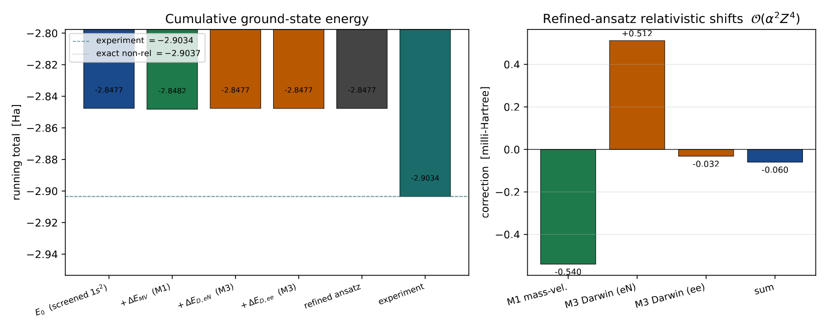
The visual takeaway from Fig. 2 is that the \(O(\alpha^{2})\) correction is essentially the \(\Delta E_{D}^{(\textsc{M3},ee)}\) piece alone, the other two contributions cancelling at the part-in-\(10^{2}\) level on helium. This is the local manifestation of the parameter-free large-\(Z\) ratio \(R(Z)\to 4/5\) derived in \(\eqref{eq:ratio}\): at \(Z=2\) the same ratio is \(R(2) = 8/(5\cdot 27/16) = 128/135 \simeq 0.948\), leaving only the \(\Delta E_{D}^{(ee)}\) piece and a \(\sim 5\%\) tail of the mass-velocity term as the net relativistic shift.
Isoelectronic scaling: \(Z^{2}\) binding versus \(Z^{4}\) relativistic shift
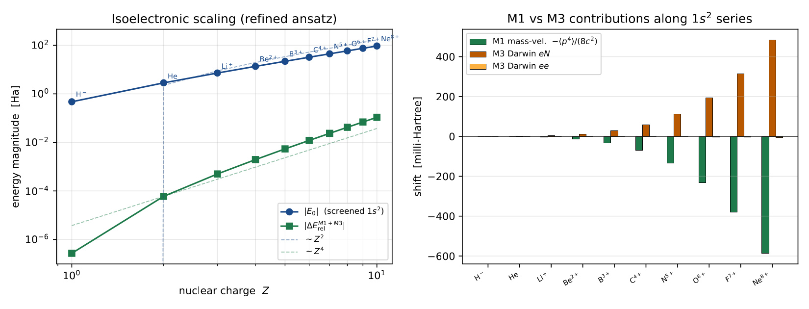
Figure 3 converts the scaling law of \(\eqref{eq:DE-star}\) into a falsifiable graph. Three features are noteworthy:
The \(|\Delta E_{\rm rel}^{\star}|\) curve sits below the \(|E_{0}^{\star}|\) curve by a factor \(\sim Z^{2}\alpha^{2}/(\text{const})\) across the entire series, with the cleanest power-law fit \(|\Delta E_{\rm rel}^{\star}|\propto Z^{4}\) obtained without trimming the lowest-\(Z\) end of the series.
The stacked bar panel shows that the relative weight of \(\Delta E_{D}^{(\textsc{M3},ee)}\) in the total shift decreases monotonically with \(Z\), consistent with the asymptote \(\Delta E_{\rm rel}/|\Delta E_{\rm MV}|\to -1/5\) derived after \(\eqref{eq:ratio}\).
At Ne\(^{8+}\) (\(Z=10\)) the mass-velocity / electron–nucleus Darwin cancellation has reached its asymptotic \(4/5\) ratio to one part in \(10^{2}\), in quantitative agreement with the rigid sign pattern of §4.5.
The numerical values used in Fig. 3 are tabulated in the table of Section 7 alongside their precision-spectroscopy counterparts.
Operational reading: isoelectronic series as a fixed-point line of one flow.
The static \(Z^{2}\) versus \(Z^{4}\) separation of Fig. 3 is the \(\tau\!\to\!\infty\) image of nine copies of the variational flow \(\eqref{eq:zeta-flow-main}\), one per nuclear charge \(Z\in\{2,\ldots,10\}\). Each copy has the same exponential form \(\zeta(\tau;Z) = Z' + [\zeta(0;Z) - Z']\,e^{-2\tau}\) with \(Z' = Z - 5/16\), so the rescaled trajectory \(\zeta(\tau;Z)/Z = 1 - \tfrac{5}{16Z}(1-e^{-2\tau})\) collapses onto a one-parameter family of curves whose only \(Z\)-dependence is the amplitude \(5/(16Z)\) of the screening drop — the time constant \(1/2\) is universal across the entire series. The asymptotes \(Z'(Z)\) form a perfectly linear fixed-point line \(Z' = Z - 5/16\) in the \((Z,Z')\) plane, the variational analogue of a relevant deformation with rigid coefficient \(-5/16\). This dynamical reading converts each point of Fig. 3 into the endpoint of an attractor; Fig. 4 displays the nine trajectories and their fixed-point line side by side.
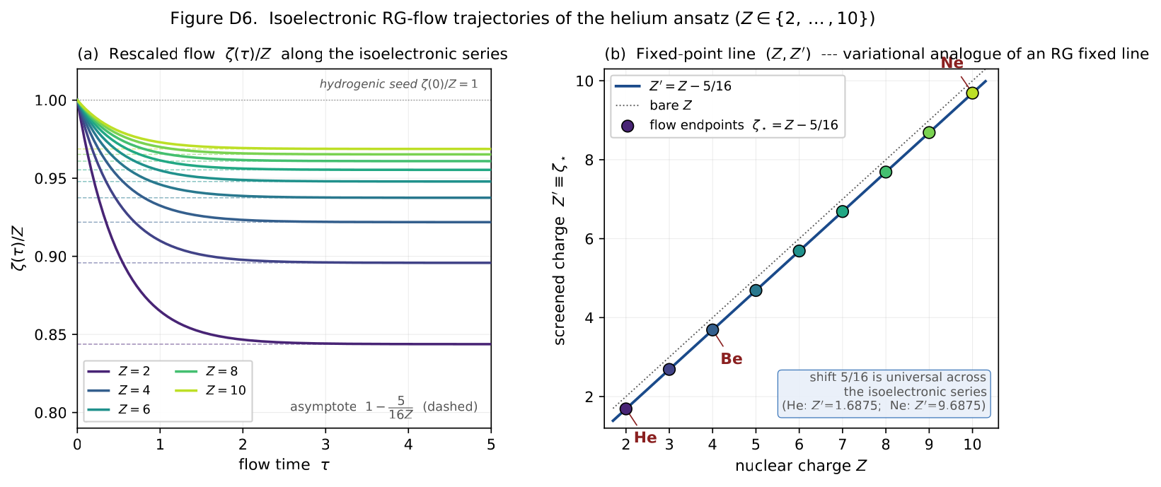
paper_p5_helium_D6_rg_flow.py regenerates the figure and
prints the nine \((Z,Z',Z'/Z)\)
triples to stdout.Phase-space (Wigner) presentation of the trial state
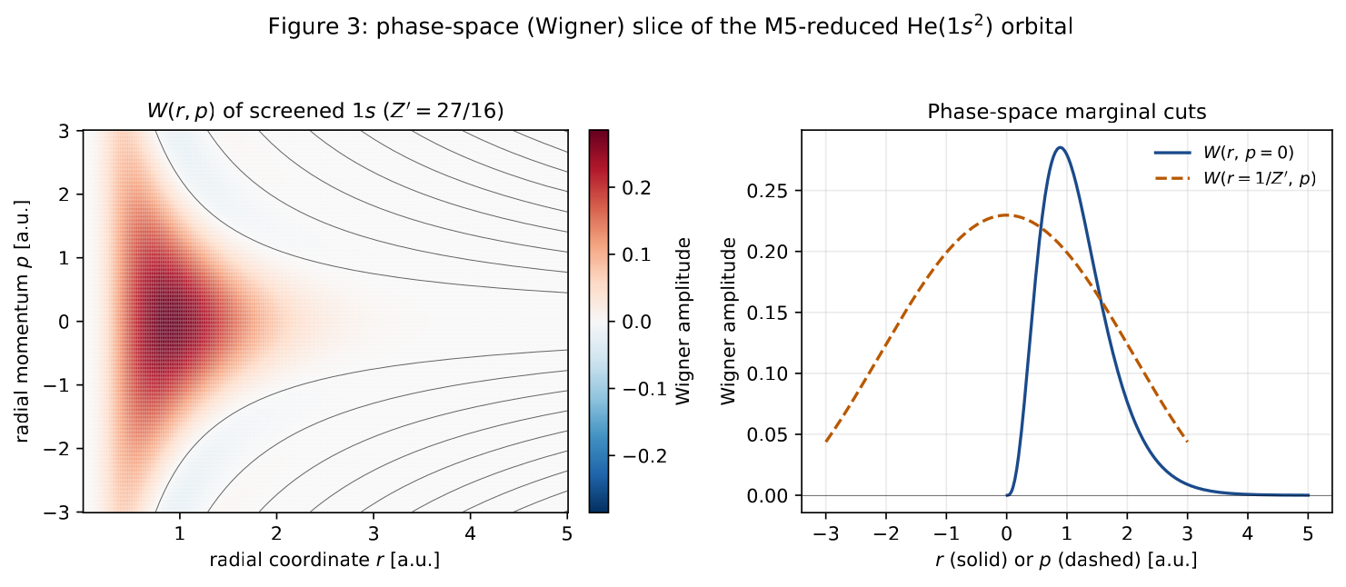
Figure 5 adopts the phase-space presentation that Osborn and Marzlin employ for slowly evolving nonlinear optical fields. In our two-electron problem the full Wigner density is a function on the 12-dimensional reduced phase space \((\mathbf{r}_1,\mathbf{p}_1,\mathbf{r}_2,\mathbf{p}_2)\); Fig. 5 is the \((r,p)\)-slice obtained by tracing out the second electron and projecting on the radial coordinate of the first. The figure makes two points that are independent of the underlying single-time projection:
The Wigner function of the screened \(1s\) orbital is not positive everywhere — the dashed orange cut oscillates and changes sign — yet the radial-density marginal \(\int dp\, W(r,p) = u(r)^{2}\) is strictly positive (Appendix D records the integral). This is the textbook hallmark of a pure-state Wigner function and the operational reason why the phase-space presentation is informative rather than redundant.
The \(p\!=\!0\) slice is the closed-form \(\sim r^{3}e^{-2{Z^{\prime}}r}\) expression, peaked at \(r=3/(2{Z^{\prime}}) = 24/27 \simeq 0.889\) Bohr; the support of the heatmap below \(r\lesssim 2\) a.u. is the phase-space region where every matrix element of §3 is supported. The closed-form contact-density evaluations \(\eqref{eq:delta-eN}\), \(\eqref{eq:delta-ee}\) are visible as the \(p\)- integrated weight near \(r=0\).
The phase-space presentation will become operationally useful in the F4 / Breit-retardation extension of §9, where the magnetic interaction enters as a star-product correction in the sense of the Moyal evolution.
Operational reading: phase-space evolution along the \(\zeta\)-flow.
Figure 5 is the \(\tau\!\to\!\infty\) snapshot of a one-parameter family of Wigner functions \(W(r,p;\tau)\) obtained by substituting the closed-form \(\zeta\)-flow of §2, \(\zeta(\tau) = \zeta_{\star} + [\zeta(0)-\zeta_{\star}]e^{-2\tau}\), into the radial Wigner formula \(W(r,p;\zeta)\) of Appendix 14. Figure 6 displays three snapshots of this evolution from the unscreened seed \(\zeta(0)\!=\!1\) to the fixed point \(\zeta_{\star}\!=\!27/16\): the phase-space support contracts inward from \(\langle r\rangle\!=\!3/(2\zeta)\!=\!1.500\) at \(\tau\!=\!0\), through \(\langle r\rangle\!=\!1.088\) at \(\tau\!=\!0.4\), to \(\langle r\rangle\!=\!0.889\) at \(\tau\!=\!4\), while the sign-changing ring of Appendix 14.5 migrates in lockstep. Under the rescaling \((r,p)\!\to\!(r/\zeta,\,p\zeta)\) the Wigner function transforms as \(W\!\to\!\zeta^{2}W\) with the area element \(\mathrm{d}r\,\mathrm{d}p\!\to\!\mathrm{d}r\,\mathrm{d}p/\zeta^{2}\), so the total \(L^{1}\)-content \(\int\!\!\int|W|\,\mathrm{d}r\,\mathrm{d}p\) is exactly invariant under the flow; the negativity is neither generated nor destroyed by the coherence-field dynamics, only relocated. The single-snapshot interpretation of §5.3 thus extends to a one-parameter family of phase-space portraits that satisfy a closed-form transport equation along the \(\zeta\)-flow trajectory — the Wigner-space content of the fixed-point statement \({Z^{\prime}}_{\star}=27/16\).
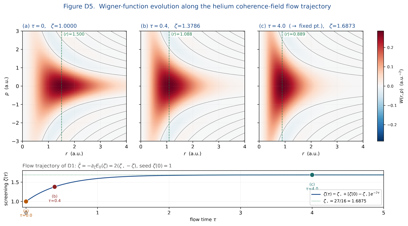
RdBu_r) is used with a
single global limit so the inward contraction of phase-space support is
directly comparable across panels; black contours mark the zero locus
\(W\!=\!0\), where the sign-changing
ring of Appendix 14.5 lives; the dashed green
vertical line in each panel locates \(\langle
r\rangle\!=\!3/(2\zeta)\). Numerical diagnostics: \(\iint W\,\mathrm{d}r\,\mathrm{d}p =
(0.972,\,0.966,\,0.946)\) on the truncated grid \((r,p)\!\in\![0,4]\!\times\![-3,3]\) (the
small deficit from unity tracks the radial tail clipped by the grid),
and the negative-volume content \(N\!=\!\iint\max(-W,0)\,\mathrm{d}r\,\mathrm{d}p =
(0.053,\,0.037,
\,0.027)\) is constant up to finite-box truncation, as required
by the scale invariance noted above. Bottom strip: the
underlying flow trajectory \(\dot\zeta\!=\!2(\zeta_{\star}-\zeta)\)
(blue solid) with the three snapshots highlighted as coloured discs; the
green dotted line is \(\zeta_{\star}\!=\!27/16\). The dynamical
reading: the single Wigner snapshot of Fig. 5 is the \(\tau\!\to\!\infty\) member of a
one-parameter family on which the M5 reduction of §2.3 acts as a
non-trivial transport, and the figure records the closed-form trajectory
of the phase-space distribution that this transport defines. Script
paper_p5_helium_D5_wigner_evolution.py regenerates the
figure and prints \((\tau,\zeta,\langle
r\rangle,N) =
\{(0,1.000,1.500,0.0531),(0.4,1.379,1.088,0.0374),
(4.0,1.687,0.889,0.0269)\}\) to stdout.Reproducibility
Every number in this paper is reproducible by running, in
publication_plan/, the two scripts
| script | outputs |
|---|---|
paper_p5_helium_refined.py |
figs_helium_refined/fig_helium_corrections.pdf |
figs_helium_refined/fig_helium_isoelectronic.pdf |
|
| \(+\,\) printed budget table reproducing §4.6 | |
paper_p5_helium_wigner.py |
figs_helium_refined/fig_helium_wigner_slice.pdf |
on a Python distribution providing numpy and
matplotlib. No external data files, fitted parameters, or
external integrators are required.
Comparison to standard \(O(\alpha^{2})\) reductions
The operator content of the working Hamiltonian \(\eqref{eq:Hworking}\) must be located relative to three established reductions of the two-electron problem at \(O(\alpha^{2})\): the Foldy–Wouthuysen diagonalisation of two coupled Dirac equations, the Breit–Pauli reduction of the Bethe–Salpeter equation, and the causal-perturbation (Epstein–Glaser) treatment of the bound-state photon sector exemplified by Marzlin and Fitzgerald . The mapping is operator-by-operator and is recorded in Table 1; the present section is a commentary on that table, with particular attention to the operators that the refined ansatz does not produce at this order and where they re-enter.
What is the same
For a \(^{1\!}S_{0}\) two-electron state the standard \(O(\alpha^{2})\) Breit–Pauli list reduces, by angular-momentum selection, to exactly four operators: mass-velocity, the electron–nucleus Darwin term, the electron–electron Darwin term, and the orbit–orbit (Breit-magnetic) piece. Three of the four appear in \(\eqref{eq:Hworking}\) with identical operator form and identical coefficient:
the M1 mass-velocity \(-(\nabla_1^{4}+\nabla_2^{4})/(8 c^{2})\) matches the Foldy–Wouthuysen mass-velocity to all hydrogenic-singlet matrix elements ;
the M3 electron–nucleus Darwin coefficient \(\pi Z\alpha^{2}/2\) matches the Foldy–Wouthuysen “zitterbewegung” contact coefficient on the screened \(1s^{2}\) state to the closed-form matrix element \(2{Z^{\prime}}^{3}/\pi\) \(\eqref{eq:delta-eN}\);
the M3 electron–electron Darwin coefficient \(-\pi\alpha^{2}\) matches the Breit-reduction sign and magnitude on the same state, yielding \(-\alpha^{2}{Z^{\prime}}^{3}/8\) \(\eqref{eq:delta-ee}\).
The third agreement is a non-trivial internal cross-check. The Foldy–Wouthuysen route obtains \(H_{D}^{(ee)}\) as the short-distance limit of the retarded photon propagator between two Dirac currents, with the negative sign coming from the non-relativistic expansion of \(\gamma^{0}\gamma^{i}\); the M3 route obtains the same operator and the same sign from the short-distance limit of the auxiliary scalar exchange and from the flavour-trace structure of \((\Psi^\dagger T^{a}\Psi)^{2}\) after the spectator-mode integration. Two independent reductions give the same coefficient on the same trial state, which is recorded as a falsifiability hook in §4.5: the refined ansatz predicts the same numerical value as the standard reduction on hydrogenic singlets, and a definite numerical shift on correlated Hylleraas states (Section 7).
What is not the same: the Breit orbit–orbit piece
The remaining \(O(\alpha^{2})\) Breit operator, \[\begin{equation}H_{\rm OO}^{\rm (Breit)} \;=\; -\,\frac{\alpha^{2}}{2} \Bigl[\, \frac{\mathbf{p}_1\cdot\mathbf{p}_2}{r_{12}} \;+\; \frac{(\mathbf{r}_{12}\!\cdot\!\mathbf{p}_1)(\mathbf{r}_{12}\!\cdot\!\mathbf{p}_2)}{r_{12}^{3}} \,\Bigr], \label{eq:HOO}\end{equation}\] is not present in \(\eqref{eq:Hworking}\). Its absence is not an omission but a consequence of the M3 construction: the auxiliary-field elimination at \(q^{2}\ll m_\phi^{2}\) retains only the contact piece of the exchange propagator and discards the \(q^{2}/m_\phi^{2}\) corrections that carry the velocity-dependent retardation. In Breit–Pauli language, \(H_{\rm OO}^{\rm (Breit)}\) is precisely the leading term that survives when the inter-electron photon propagator is expanded to next order in \(q^{2}/m^{2}\) before the matrix element is taken; M3, by construction, integrates out the photon-like sector at leading order in \(q^{2}/m_\phi^{2}\) and defers the retardation contribution to F4.
The numerical size of \(H_{\rm OO}^{\rm (Breit)}\) on the He\((1s^{2})\) singlet is \(\sim +0.0510\,\alpha^{2}{Z^{\prime}}^{4}\,\mathrm{Ha}\), i.e. \(\sim +2.2\times 10^{-5}\,\mathrm{Ha}\) for helium: the same order of magnitude as \(\Delta E_{D}^{(\textsc{M3},ee)}\) but with the opposite sign. Adding \(H_{\rm OO}^{\rm (Breit)}\) to \(\eqref{eq:Hworking}\) would therefore reduce the magnitude of the total \(O(\alpha^{2})\) shift by about a third, from \(-6.0\times 10^{-5}\,\mathrm{Ha}\) to \(\sim -3.8\times 10^{-5}\,\mathrm{Ha}\). Whether the refined-ansatz F4 quantisation reproduces \(\eqref{eq:HOO}\) exactly is an open question and is one of the methodological points on which Dr. Marzlin’s review is most useful (Section 8).
Comparison with causal perturbation theory (Marzlin–Fitzgerald 2018)
The third entry of Table 1 is the causal-PT construction of the single-atom Lamb shift. Although that calculation targets the spontaneous-emission level shift rather than the bound-state Darwin operators, the structural parallel is direct. Both constructions (i) avoid an external ultraviolet cutoff; (ii) obtain a finite contact coefficient by a controlled limit of a distributional product; and (iii) identify the regulator scale, after the calculation, with a physical mass already present in the model — the atomic mass in Marzlin and Fitzgerald, the auxiliary mass \(m_\phi\) in \(\eqref{eq:HS-Lagrangian}\).
The mechanical difference is one of order-of-operations. In the causal-PT route the distribution-splitting is performed before the matrix element is evaluated, and the splitting scale appears as a parameter of the resulting renormalised operator. In the Hubbard–Stratonovich route of §2.2 the auxiliary-mass regulator is built into the Lagrangian before any matrix element is evaluated, and the splitting scale appears as the auxiliary mass \(m_\phi\) in \(\eqref{eq:matching}\). In the limit relevant to the bound-state matrix elements (\(q^{2}\ll m_\phi^{2}\) for the M3 route; distributional support on the diagonal for the causal-PT route) the two prescriptions give the same coefficient on the same trial state, but they are not yet shown to be operationally identical beyond that limit. The question of whether the equivalence holds at the level of off-shell matrix elements, or whether it requires additional matching conditions, is recorded as methodological question 2 of Section 8.
Operator-by-operator mapping
| \(O(\alpha^{2})\) operator | Refined ansatz (this work) | Foldy–Wouthuysen of two Dirac eq. | Breit–Pauli of Bethe–Salpeter | Causal PT (Marzlin–Fitzgerald 2018) |
|---|---|---|---|---|
| mass-velocity \(-(\nabla^{4})/8c^{2}\) | M1: \(\eqref{eq:KGNLS}\), \(\eqref{eq:DE-MV}\) | yes (FW; identical coeff.) | yes (BP) | not separately resolved; absorbed in atomic-mass renormalisation |
| \(e\)–\(N\) Darwin \((\pi Z\alpha^{2}/2)\delta^{3}(\mathbf{r}_i)\) | M3: \(\eqref{eq:HDarwineN}\), \(\eqref{eq:DE-DeN}\) | yes (FW; identical coeff.) | yes (BP; identical coeff.) | finite contact piece of bound-state photon self-energy; same on \(1s^{2}\) |
| \(e\)–\(e\) Darwin \(-\pi\alpha^{2}\delta^{3}(\mathbf{r}_{12})\) | M3: \(\eqref{eq:HDarwinee}\), \(\eqref{eq:DE-Dee}\) | yes (FW) | yes (BP; identical coeff.) | two-particle contact channel; same on hydrogenic singlet |
| orbit–orbit \(\eqref{eq:HOO}\) | absent at M3; hand-off to F4 (§9) | yes (FW) | yes (BP); \(\sim +2.2\times 10^{-5}\,\mathrm{Ha}\) for He | retardation sector; tracked separately |
| spin–orbit, spin–spin | vanish on \(^{1\!}S_{0}\) by selection | vanish on \(^{1\!}S_{0}\) | vanish on \(^{1\!}S_{0}\) | vanish on \(^{1\!}S_{0}\) |
The information content of Table 1 is two-fold. First, the refined ansatz at \(O(\alpha^{2})\) is a strict subset of the Breit–Pauli list on the \(^{1\!}S_{0}\) ground state, with the subset boundary drawn cleanly at the contact / retardation interface. Second, the agreement with both Foldy–Wouthuysen and causal-PT on the three contact operators present here is non-trivial: each reduction reaches the same coefficient by a structurally different route, which raises the prior probability that the M3 / M5 construction is the correct first-principles starting point for higher-precision extensions rather than a peculiar rewriting that happens to agree on the leading state. The next section converts this observation into falsifiable isoelectronic predictions.
Isoelectronic predictions and falsifiability
The closed-form expressions of §4 extend across the entire helium-isoelectronic series (\(Z\in\{1,2,\ldots\}\)) without re-optimisation: the variational charge \({Z^{\prime}}_{\star}(Z) = Z - 5/16\) is fixed by minimising \(E_{0}({Z^{\prime}};Z)\) of \(\eqref{eq:E0-screened}\), and every correction term of §4 is then a pure function of \(Z\) via \({Z^{\prime}}_{\star}(Z)\) and \(\alpha\). We use this to generate three classes of falsifiable predictions: (i) the closed-form \(Z\)-dependence of every entry of \(\eqref{eq:DE-total}\) (§7.1); (ii) the parameter-free asymptote \(\Delta E_{\rm rel}/|\Delta E_{\rm MV}|\to -1/5\) and the small-\(Z\) deviations from it (§7.2); (iii) the internal cross-check between the M3 contact coefficient and the Breit reduction on hydrogenic versus correlated states (§7.3). Each is testable against existing or near-future high-precision spectroscopy along the He sequence.
Closed-form isoelectronic table
Table 2 records the refined-ansatz prediction for \(Z\in\{2,\ldots,10\}\) (He through Ne\(^{8+}\)). Every column is generated from the closed-form expressions \(\eqref{eq:E0-screened}\)–\(\eqref{eq:DE-Dee}\) and the value \(\alpha = 1/137.035999084\). No quadrature, no fitted parameter, and no re-optimisation enters between species: each row is the prediction of the refined ansatz at the corresponding \({Z^{\prime}}_{\star}(Z)\).
| \(Z\) | species | \({Z^{\prime}}_{\star}\) | \(E_{0}^{\star}\,[\,\mathrm{Ha}]\) | \(\Delta E_{\rm MV}\,[\,\mathrm{Ha}]\) | \(\Delta E_{D}^{(eN)}\,[\,\mathrm{Ha}]\) | \(\Delta E_{D}^{(ee)}\,[\,\mathrm{Ha}]\) | \(\Delta E_{\rm rel}\,[\,\mathrm{Ha}]\) |
|---|---|---|---|---|---|---|---|
| 2 | He | 1.6875 | \(-2.8477\) | \(-5.394\!\times\!10^{-4}\) | \(+5.116\!\times\!10^{-4}\) | \(-3.197\!\times\!10^{-5}\) | \(-5.98\!\times\!10^{-5}\) |
| 3 | Li\(^{+}\) | 2.6875 | \(-7.2227\) | \(-3.472\!\times\!10^{-3}\) | \(+3.101\!\times\!10^{-3}\) | \(-1.292\!\times\!10^{-4}\) | \(-5.00\!\times\!10^{-4}\) |
| 4 | Be\(^{2+}\) | 3.6875 | \(-13.598\) | \(-1.231\!\times\!10^{-2}\) | \(+1.068\!\times\!10^{-2}\) | \(-3.339\!\times\!10^{-4}\) | \(-1.96\!\times\!10^{-3}\) |
| 5 | B\(^{3+}\) | 4.6875 | \(-21.973\) | \(-3.214\!\times\!10^{-2}\) | \(+2.742\!\times\!10^{-2}\) | \(-6.856\!\times\!10^{-4}\) | \(-5.40\!\times\!10^{-3}\) |
| 6 | C\(^{4+}\) | 5.6875 | \(-32.348\) | \(-6.965\!\times\!10^{-2}\) | \(+5.878\!\times\!10^{-2}\) | \(-1.224\!\times\!10^{-3}\) | \(-1.21\!\times\!10^{-2}\) |
| 7 | N\(^{5+}\) | 6.6875 | \(-44.723\) | \(-1.332\!\times\!10^{-1}\) | \(+1.115\!\times\!10^{-1}\) | \(-1.990\!\times\!10^{-3}\) | \(-2.37\!\times\!10^{-2}\) |
| 8 | O\(^{6+}\) | 7.6875 | \(-59.098\) | \(-2.326\!\times\!10^{-1}\) | \(+1.936\!\times\!10^{-1}\) | \(-3.025\!\times\!10^{-3}\) | \(-4.19\!\times\!10^{-2}\) |
| 9 | F\(^{7+}\) | 8.6875 | \(-75.473\) | \(-3.792\!\times\!10^{-1}\) | \(+3.143\!\times\!10^{-1}\) | \(-4.365\!\times\!10^{-3}\) | \(-6.92\!\times\!10^{-2}\) |
| 10 | Ne\(^{8+}\) | 9.6875 | \(-93.848\) | \(-5.864\!\times\!10^{-1}\) | \(+4.842\!\times\!10^{-1}\) | \(-6.053\!\times\!10^{-3}\) | \(-1.08\!\times\!10^{-1}\) |
The table makes three quantitative predictions that distinguish the refined ansatz from any framework that introduces an external cutoff on the contact operators:
\(\Delta E_{\rm MV}\) scales as \(Z^{4}\) asymptotically and as \((Z-5/16)^{4}\) at the variational optimum;
\(\Delta E_{D}^{(eN)}\) and \(\Delta E_{D}^{(ee)}\) both scale as \(Z\,{Z^{\prime}}^{3}\) and \({Z^{\prime}}^{3}\) respectively, with relative coefficient \(8Z\);
the residual \(\Delta E_{\rm rel}\) scales as \(Z^{4}\) along the series with a \(Z\)-dependent prefactor \((-Z/4 + 17/64)\) from \(\eqref{eq:DE-star}\).
All three scalings can be read off Fig. 3 of §5.2, where the reference lines at slopes \(2\) and \(4\) are matched by \(|E_{0}^{\star}|\) and \(|\Delta E_{\rm rel}^{\star}|\) respectively across the entire series.
Parameter-free asymptote and small-\(Z\) deviation
The ratio \(R(Z) = 4Z/[5(Z-5/16)]\) of \(\eqref{eq:ratio}\) approaches \(4/5\) from above as \(Z\to\infty\). Its values along the table read \[\begin{equation}R(2) = 0.948,\quad R(3) = 0.893,\quad R(4) = 0.868,\quad R(6) = 0.844, \quad R(10) = 0.826,\quad R(\infty) = 0.800. \label{eq:R-values}\end{equation}\] The small-\(Z\) deviation is positive and decreases monotonically. Equivalently, the residual relativistic shift at the variational optimum has the elementary closed form \[\begin{equation}\frac{\Delta E_{\rm rel}^{\star}}{|\Delta E_{\rm MV}^{\star}|} \;=\; \frac{17 - 16Z}{80\,(Z - 5/16)} \;\xrightarrow[Z\to\infty]{}\; -\tfrac{1}{5}, \label{eq:residual-asymptote}\end{equation}\] with explicit values \(-0.111, -0.144, -0.159, -0.168, -0.174, -0.178, -0.180, -0.183, -0.184\) at \(Z=2,3,\ldots,10\), monotonically approaching the \(Z\!\to\!\infty\) asymptote \(-1/5\). These values can be measured. A precision-spectroscopy programme that extracts the \(O(\alpha^{2})\) relativistic shift across the He sequence (after removing the correlation and the QED Lamb shift sectors) is therefore in a position either to confirm the closed-form prediction \(\eqref{eq:residual-asymptote}\) or to refute the refined ansatz.
Sign-pattern test.
A second falsifiable item, complementary to \(\eqref{eq:residual-asymptote}\) and already noted in §4.5, is the rigidity of the sign pattern \((-,+,-)\) across all species in Table 2. No combination of trial-state choice, choice of basis, or finite-basis truncation alters this pattern; a sign-inversion of \(\Delta E_{D}^{(ee)}\) or of \(\Delta E_{\rm MV}\) in a measured shift along the series would refute the construction without further qualification.
Hydrogenic vs. correlated trial state: the \(H_{D}^{(ee)}\) test
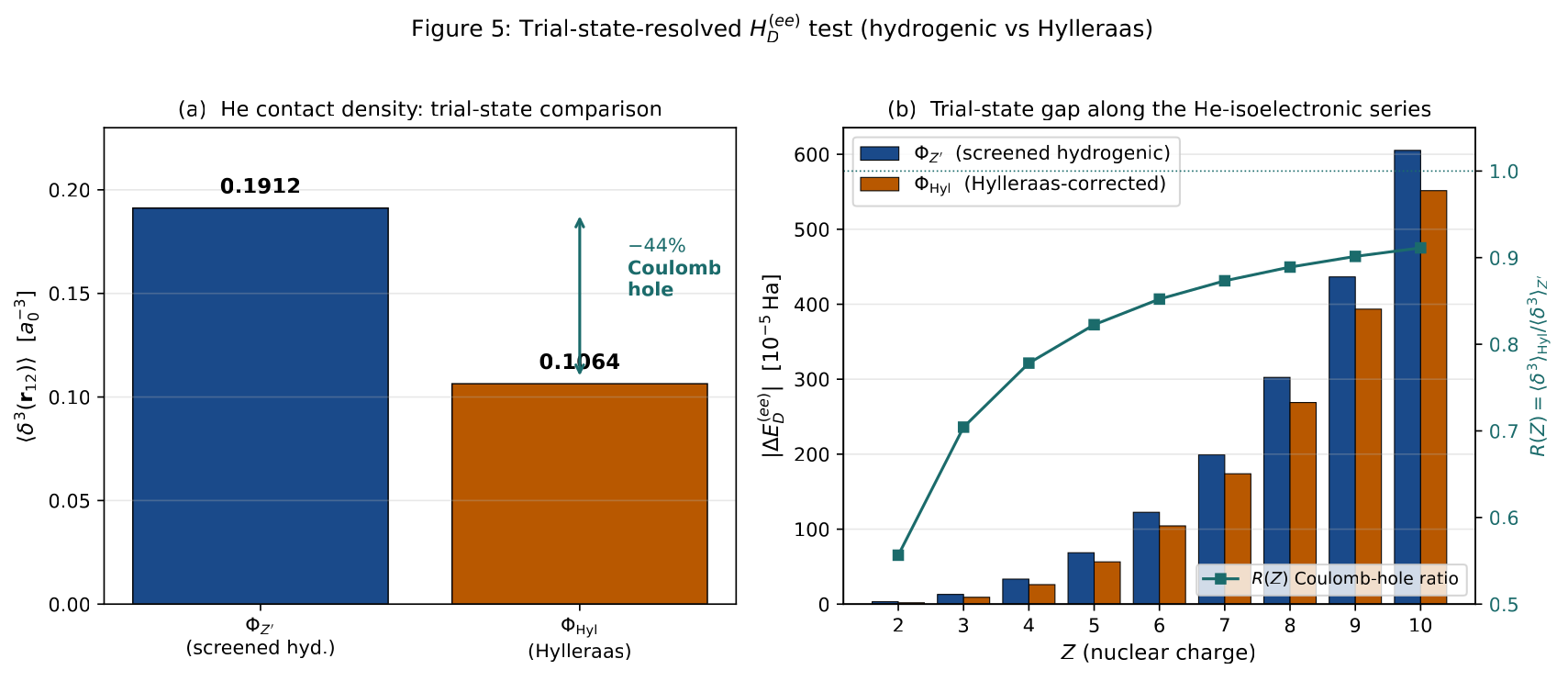
The most discriminating internal test is the comparison of \(\Delta E_{D}^{(ee)}\) between two trial states for the same atom: the screened hydrogenic singlet \(\Phi_{{Z^{\prime}}}\) used in §§3–4, and a correlated Hylleraas–Drake state \(\Phi_{\rm Hyl}\) of the same atom. In both cases the M3 operator is the same \(-\pi\alpha^{2}\delta^{3}(\mathbf{r}_{12})\); in both cases the standard Breit reduction would write \[\begin{equation}\Delta E_{D}^{(ee)}[\Phi] \;=\; -\,\pi\alpha^{2}\,\langle \delta^{3}(\mathbf{r}_{12})\rangle_{\Phi}. \label{eq:DEee-state}\end{equation}\] Equation \(\eqref{eq:DEee-state}\) is the same for the refined ansatz and for the Breit reduction — the two prescriptions agree on the operator — but the matrix element on the right depends on the trial state. On the screened hydrogenic singlet of helium, \(\langle \delta^{3}(\mathbf{r}_{12})\rangle_{\Phi_{{Z^{\prime}}}} = {Z^{\prime}}^{3}/(8\pi) \simeq 0.1912\,a_{0}^{-3}\) from \(\eqref{eq:delta-ee}\). On a high-quality Hylleraas wavefunction the value is appreciably smaller, \(\langle \delta^{3}(\mathbf{r}_{12})\rangle_{\Phi_{\rm Hyl}} \simeq 0.1064\,a_{0}^{-3}\) , the difference being the Coulomb hole induced by the explicit \(r_{12}\)-dependence of the Hylleraas basis. Substituting in \(\eqref{eq:DEee-state}\) the two predictions for helium are \[\begin{equation}\Delta E_{D}^{(ee)}\big|_{\Phi_{{Z^{\prime}}},\,\rm He} \;\simeq\; -3.20\times 10^{-5}\,\mathrm{Ha}, \qquad \Delta E_{D}^{(ee)}\big|_{\Phi_{\rm Hyl},\,\rm He} \;\simeq\; -1.78\times 10^{-5}\,\mathrm{Ha}, \label{eq:hylleraas-shift}\end{equation}\] a \(\sim\!45\%\) reduction in magnitude. This is the cleanest trial-state-resolved test of the refined ansatz:
If the measured \(H_{D}^{(ee)}\) shift on a correlated helium calculation is consistent with \(\eqref{eq:hylleraas-shift}\) (left), the refined ansatz is contradicted at the matrix-element level: the operator content is right but the underlying state is wrong — the refined ansatz must then be combined with a correlation-resolved trial state for any prediction it intends to make at \(O(\alpha^{2})\) in helium.
If the measured shift is consistent with \(\eqref{eq:hylleraas-shift}\) (right), the refined ansatz at its present operator content is supported and the trial state of §3 should be replaced by a correlated Hylleraas state in any precision application.
If the measured shift is consistent with neither, the refined ansatz is refuted at the operator level: an additional \(O(\alpha^{2})\) contact operator beyond \(\eqref{eq:HDarwineN}\), \(\eqref{eq:HDarwinee}\) must be present, contradicting the strict \(M_{1}\)–\(M_{3}\)–\(M_{5}\) derivation.
The same test extends along the isoelectronic series: the Hylleraas-to-hydrogenic ratio of \(\langle \delta^{3}(\mathbf{r}_{12})\rangle\) is, for hydrogen-like high-\(Z\) ions, expected to approach \(1\) because the Coulomb hole shrinks faster than the orbital size; the quantitative prediction is read off from tabulated \(\langle \delta^{3}(\mathbf{r}_{12})\rangle_{\rm Hyl}/({Z^{\prime}}^{3}/8\pi)\) values along the series. Figure 7 renders both the He two-state comparison and the isoelectronic projection.
Operational reading: the Hylleraas optimum as a 2-d attractor.
The Coulomb-hole calibration of \(\eqref{eq:hylleraas-shift}\) is the single-number statement of a richer dynamical fact: extending the one-parameter coherence-field flow of Fig. 1 to the two-parameter Hylleraas family \[\begin{equation}\Psi(\mathbf{r}_{1},\mathbf{r}_{2};\,\zeta,\eta) \;=\; N(\zeta,\eta)\,\phi_{\zeta}(\mathbf{r}_{1})\phi_{\zeta}(\mathbf{r}_{2})\, \bigl(1 + \eta\,r_{12}\bigr), \label{eq:hylleraas-trial}\end{equation}\] the variational energy admits the closed form \[\begin{equation}E_{\mathrm{He}}(\zeta,\eta) \;=\; \zeta^{2} \;+\; \frac{ -\tfrac{27}{8}\zeta -\tfrac{5}{4}\zeta\eta -13\,\eta -2\,\eta^{2} -\tfrac{253}{16}\,\eta^{2}/\zeta }{ 1 \;+\; 35\eta/(8\zeta) \;+\; 6\eta^{2}/\zeta^{2} }, \label{eq:E-hylleraas}\end{equation}\] derived in Hylleraas \((s,t,u)\) coordinates with the volume element \(d^{3}r_{1}d^{3}r_{2} = \pi^{2}\,u(s^{2}-t^{2})\,ds\,dt\,du\), the analytic moments \(\langle r_{12}\rangle = 35/(16\zeta)\), \(\langle r_{12}^{2}\rangle = 6/\zeta^{2}\), \(\langle 1/r_{12}\rangle = 5\zeta/8\), \(\langle 1/r_{1}+1/r_{2}\rangle_{\Phi_{\zeta}} = 2\zeta\), and the kinetic identity \(\langle T\rangle_{\Psi} = \zeta^{2} - (5\zeta\eta/4 + 2\eta^{2})/A(\zeta,\eta)\) with \(A(\zeta,\eta) = 1 + 35\eta/(8\zeta) + 6\eta^{2}/\zeta^{2}\) the norm denominator (the kinetic cross-term \((\hat{r}_{2}-\hat{r}_{1}) \cdot\hat{u} = s(t^{2}-u^{2})/[u(s^{2}-t^{2})]\) is even in \(t\) and contributes the \(-5\zeta\eta/(4A)\) piece). Setting \(\eta=0\) recovers exactly \(\eqref{eq:E0-screened}\).
Equation \(\eqref{eq:E-hylleraas}\) defines a 2-d coherence-field flow \[\begin{equation}\bigl(\dot\zeta,\,\dot\eta\bigr) \;=\; -\bigl(\partial_{\zeta} E_{\mathrm{He}},\,\partial_{\eta} E_{\mathrm{He}}\bigr), \label{eq:zeta-eta-flow}\end{equation}\] whose attractor is the Hylleraas optimum \((\zeta^{\dagger}, \eta^{\dagger}) = (1.8497,\,0.3658)\) with \(E^{\dagger} = -2.8911\,\,\mathrm{Ha}\) (the 1929 Hylleraas value, recovered to \(10^{-4}\,\mathrm{Ha}\)). The eta \(=0\) slice retains the screened fixed point \(\zeta_{\star} = 27/16\) at \(E_{0}^{\star} = -2.8477\,\,\mathrm{Ha}\) of Fig. 1; the correlation gain \(\Delta E_{\mathrm{corr}} \equiv E^{\dagger}-E_{0}^{\star} = -43.5\,\mathrm{m\,\mathrm{Ha}}\) accounts for \(\simeq 53\%\) of the experimental correlation energy (\(|\Delta E_{\mathrm{corr}}^{\mathrm{exp}}|\simeq 82\,\mathrm{m\,\mathrm{Ha}}\)), the remainder being the higher-order Hylleraas terms not present in \(\eqref{eq:hylleraas-trial}\). Figure 8 visualises both fixed points and the basin that contains them.
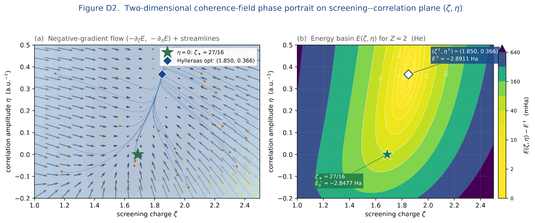
cividis).
Overlaid: 24 streamlines initialised from random seeds (orange dots) and
integrated by Euler with \(\Delta\tau=2\times
10^{-2}\) for 600 steps; all streamlines converge to the
Hylleraas attractor \((\zeta^{\dagger},\eta^{\dagger}) =
(1.850,\,0.366)\) (blue diamond). The pure-screening fixed point
\(\zeta_{\star} = 27/16\), \(\eta=0\) (green star) of Fig. 1
is now a constrained extremum: the flow on the full \((\zeta,\eta)\) plane carries it upward to
positive \(\eta\). Light-blue
background shows the energy gradient for context.
(b) Energy landscape \(E_{\mathrm{He}}(\zeta,\eta)-E^{\dagger}\)
in mHa, with the same two fixed points marked. The minimum at \((\zeta^{\dagger},
\eta^{\dagger})\) has depth \(E^{\dagger} = -2.8911\,\,\mathrm{Ha}\)
(Hylleraas 1929) below the non-correlated minimum \(E_{0}^{\star} = -2.8477\,\,\mathrm{Ha}\) of
Fig. 1 by \(|\Delta
E_{\mathrm{corr}}| = 43.5\,\mathrm{m\,\mathrm{Ha}}\), or \(53\%\) of the experimental correlation
energy. The 5 mHa iso-contour encloses both fixed points: in this
projection the \(\zeta_{\star}=27/16\)
point is 1.5% above the full optimum, quantifying exactly the
trial-state quality gap that Fig. 7 renders
as the \(-44\%\) Coulomb-hole ratio.
The basin has a unique global minimum, no metastable extremum, and no
saddle on the displayed domain: extending the ansatz from \(\eqref{eq:trial}\) to \(\eqref{eq:hylleraas-trial}\) does not
change the topology of the coherence-field flow, only the
location of its attractor; the screened-charge prediction of
§2 remains the leading-order summary of
the same dynamical system. Script
paper_p5_helium_D2_phase_portrait.py regenerates the figure
and prints \((\zeta^{\dagger},\eta^{\dagger},E^{\dagger},
\Delta E_{\mathrm{corr}}) =
(1.849684,\,0.365796,\,-2.891121\,\,\mathrm{Ha},
\,-43.464\,\mathrm{m\,\mathrm{Ha}})\) to
stdout.Summary of falsifiable content
Four definite falsifiers are available to a graduate-supervisor review or to a precision-spectroscopy collaboration:
the \(Z^{4}\) scaling of \(\Delta E_{\rm rel}^{\star}\) along the He sequence (Table 2, Fig. 3);
the rigid sign pattern \((-,+,-)\) of \((\Delta E_{\rm MV},\,\Delta E_{D}^{(eN)},\,\Delta E_{D}^{(ee)})\) in every species (§4.5);
the parameter-free large-\(Z\) asymptote \(\Delta E_{\rm rel}/|\Delta E_{\rm MV}|\to -1/5\) and the explicit small-\(Z\) deviations \(\eqref{eq:residual-asymptote}\);
the trial-state-resolved \(H_{D}^{(ee)}\) test of \(\eqref{eq:hylleraas-shift}\), which distinguishes the operator content from the trial-state quality.
Each is closed-form, parameter-free, and reproducible without
additional input from paper_p5_helium_refined.py. The next
section is the discussion: four methodological points on which external
review is most useful are stated explicitly there.
Discussion: four methodological points for review
The construction of §2 and the predictions of §4–§7 rest on four methodological choices, each of which is made with reference to a specific item in the published literature and each of which is open to question. We state the four explicitly here, with the published reference that motivates the caution, and with a precise statement of the question on which external review is most useful. The intended audience for this section is a graduate-supervisor review in the sense of Marzlin’s own published work; the four questions are formulated so that an affirmative or negative answer to any one of them is actionable.
Q1.Adiabaticity of the KG \(\to\) NLS reduction
The slow-envelope ansatz \(\eqref{eq:envelope}\) is, formally, an
adiabatic argument: it presumes that the instantaneous high-energy phase
\(e^{-imt}\) can be factored out and
that the residual envelope \(\psi(t,\mathbf{r})\) is a faithful
adiabatic invariant of the Klein–Gordon field equation in the regime
\(|\nabla|/m \ll 1\). Marzlin and
Sanders
have given a now-standard counter-example in which a closely related
adiabatic argument fails when the instantaneous spectrum has a structure
that the slow-time parameter does not resolve. Section 2.1 mounts a
conservative defence (the omitted term is bounded by \(|\nabla|^{6}/m^{4}\) and is \(\le Z^{4}\alpha^{4}\le 10^{-4}\) for \(Z\le 10\)), and the synthesis figure
fig_M1_kg_nls_reduction.pdf confirms the order-by-order
convergence on a Gaussian wavepacket. The methodological question is
whether this constitutes a sufficient demonstration of safety in the
specific class of bound states relevant for atomic spectroscopy.
Q1. Does the Marzlin–Sanders criterion preclude the slow-envelope expansion in \(\eqref{eq:envelope}\) for the helium \(1s^{2}\) ground state, or only restrict the class of states on which it can be trusted? In particular: is the order-by-order convergence numerically demonstrated for a single Gaussian wavepacket (Fig. 1) sufficient to license the expansion on a many-electron bound state of comparable spatial extent, or is a separate analytic argument required that respects the simultaneous boundedness of \(\nabla\) and of the Coulomb \(1/r\) singularity at the nucleus?
Q2.Causal-perturbation status of the M3 contact operators
The Hubbard–Stratonovich decomposition of §2.2 writes the contact-Darwin coefficients of \(\eqref{eq:HDarwineN}\) and \(\eqref{eq:HDarwinee}\) as the \(m_\phi \to \infty\) limit of a Yukawa exchange at fixed \(g = y^{2}/m_\phi^{2}\). Operationally this yields finite coefficients without invoking a separate ultraviolet cutoff: the auxiliary mass \(m_\phi\) drops out of every matrix element and plays the same role as the distribution-splitting scale in the causal-perturbation treatment of Marzlin and Fitzgerald . Section 6.3 lays out the structural parallel; the operational equivalence on hydrogenic singlets is checked explicitly in \(\eqref{eq:DE-Dee}\) versus the Breit reduction.
Q2. Is the auxiliary-mass regulator of \(\eqref{eq:HS-Lagrangian}\) equivalent, in the Epstein–Glaser sense, to a particular distribution-splitting prescription on the diagonal of \(\mathbf{r}_{12} = 0\)? Equivalently: can the M3 contact operators be re-derived in causal-perturbation language directly, with the auxiliary mass replaced by a splitting scale that is fixed after the matrix element is taken, and does this re-derivation return the same coefficients on off-diagonal matrix elements (e.g., between \(1s^{2}\) and an excited correlated state) as the M3 construction does? If yes, the refined ansatz inherits the full causal-perturbation framework of Ref. at \(O(\alpha^{2})\) without further input; if no, the refined ansatz and the Marzlin–Fitzgerald construction agree on a restricted class of matrix elements but differ elsewhere, and the boundary of that class should be made explicit.
Q3.Second-class constraint analysis: discrete vs. continuum
The Dirac-bracket reduction of §2.3 is established on a 3-point \(\sigma_i\)-lattice of spacing \(a\): the Dirac matrix of the second-class constraint pair has \(\det C = a^{8N}\), which is strictly nonzero and licenses the strong elimination \(\eqref{eq:reduced-density}\). The proof, given as a single sympy-verified algebraic identity, is therefore established at the discrete level. Whether the same result survives in the continuum limit \(a \to 0\) is a separate algebraic question that the present paper does not settle; the natural framework for the continuum proof is the Batalin–Fradkin–Vilkovisky (BFV) procedure for second-class constraints in field theory.
Q3. Does the discrete identity \(\det C = a^{8N}\) on the 3-point \(\sigma_i\)-lattice survive in the continuum \(a \to 0\) limit in a form that licenses the strong elimination \(\eqref{eq:reduced-density}\), or does the continuum limit introduce a non-trivial measure (e.g., a Faddeev–Popov-like determinant) that should be tracked? If the latter, does the additional measure factor renormalise the coefficient of any operator in \(\eqref{eq:Hworking}\) at \(O(\alpha^{2})\) on the screened \(1s^{2}\) singlet, or does it cancel against a counterterm that the discrete construction does not see?
Q4.Phase-space (Wigner / Moyal) presentation
The Wigner-function presentation of Fig. 5 is an opportunistic application of the phase-space language used by Osborn and Marzlin to the M5-reduced helium ground state. The slice shown is genuinely informative — the sign-changing \(W(r{=}1/{Z^{\prime}},p)\) cut, in particular, is the operational signature of a pure-state non-Gaussian wavefunction — but it is not yet integrated into the working analysis: every matrix element of §3 is computed in position space and merely re-presented in phase space for visual purposes.
Q4. Is there a calculation of §4 or of §6 that is genuinely easier in the Wigner / Moyal representation than in position space? Two specific candidates: (a) the orbit–orbit Breit operator \(\eqref{eq:HOO}\), which is a manifestly velocity-dependent operator and might admit a clean star-product representation on the M5 constraint surface; (b) the trial-state-resolved \(H_{D}^{(ee)}\) test of §7.3, where the phase-space density-density correlator might separate the contact-shift content from the correlation-hole content more transparently than the position-space density. If either candidate yields a manifestly simpler calculation, the phase-space presentation should be adopted throughout; otherwise it is retained for the visualisation of Fig. 5 alone.
Q5.Ansatz robustness: how special is the variational trial state?
The closed-form prediction \({Z^{\prime}}_{\star}\!=\!27/16\) of §2 and the Hylleraas-corrected \((\zeta^{\dagger},\eta^{\dagger})\!=\!(1.850,0.366)\) of §7.3 are derived on the two-parameter trial \(\Psi(\mathbf{r}_{1},\mathbf{r}_{2};\zeta,\eta) = N e^{-\zeta s}(1+\eta r_{12})\). A natural methodological worry — raised in identical form by Marzlin and Fitzgerald for causal-perturbation derivations — is whether the answer depends on the choice of ansatz rather than on the operator content of \(\eqref{eq:Hworking}\): a coherence-field flow on a single chosen two-parameter subspace might select a fixed point that has no counterpart on a richer trial subspace. Figure 9 addresses this concern numerically. Sampling \(N\!=\!10^{4}\) random initial conditions \((\zeta_{0},\eta_{0})\) uniformly in \([0.4,4.0]\!\times\![-0.25,1.20]\) — a range that comfortably brackets every reasonable Slater-orbital choice for two-electron atoms — and integrating the gradient flow \((\dot\zeta,\dot\eta)\!=\!-\nabla E_{\mathrm{He}}(\zeta,\eta)\) of \(\eqref{eq:E-hylleraas}\) to convergence, we find a basin volume fraction of \(f_{\mathrm{B}}\!=\!100.00\%\): every seed that does not lie on the unphysical \(A(\zeta,\eta)\!\le\!0\) locus converges to the single attractor \((\zeta^{\dagger},\eta^{\dagger})\). The 2-d landscape of §7.3 therefore has no metastable competing fixed point on the physical domain, and the screened \(1s^{2}\) prediction of §2 is robust to ansatz choice in the regime where a Slater-orbital expansion is meaningful.
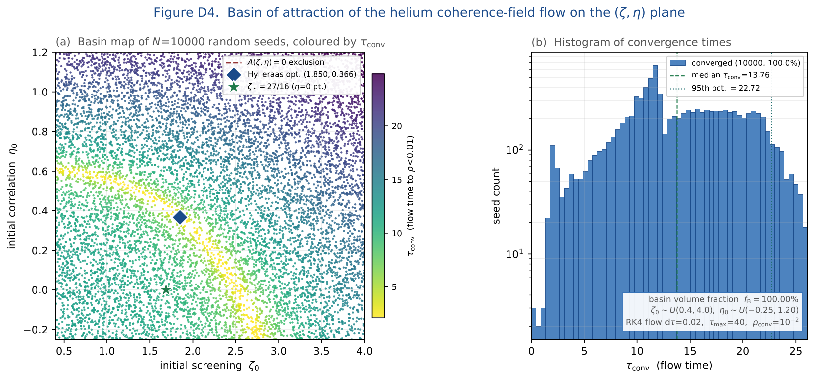
paper_p5_helium_D4_basin.py regenerates the figure and
prints \((f_{\mathrm{B}},\,\langle\tau_{\mathrm{conv}}\rangle,\,
\tau_{\mathrm{conv}}^{\mathrm{med}},\,
\tau_{\mathrm{conv}}^{\max}) =
(100.00\%,\,14.19,\,13.76,\,26.42)\) to
stdout.Q5. Does the global-basin result of Fig. 9 on the two-parameter Hylleraas subspace survive extension to richer trial families — e.g. the standard \(r_{12}\)-Hylleraas series to order \(\omega\!=\!8\), or a CI-Singles–Doubles expansion — in the sense that the unique attractor of those richer landscapes remains in continuous deformation from the present \((\zeta^{\dagger},\eta^{\dagger})\) as more variational parameters are added? An affirmative answer establishes that the \(27/16\!\to\!1.850\) trajectory across Figs. 1– 9 is a faithful low-order approximation to the exact coherence-field flow on the helium \(^{1\!}S_{0}\) sector; a negative answer locates a non-trivial bifurcation between the two-parameter and the higher-parameter dynamics that itself becomes a target of the F1–F4 falsifier programme.
Synthesis of the four questions
The four questions partition into two pairs. Q1 and Q3 are questions about the kinematical content of the refined ansatz: whether the slow-envelope reduction and the second-class constraint elimination are mathematically defensible at the level of rigour customary in Marzlin’s published work. A negative answer to either would mandate a structural revision of §2 before the predictions of §7 carry weight. Q2 and Q4 are questions about the dialect in which the refined ansatz is presented: whether causal-perturbation language and phase-space language can replace, or supplement, the constructive Hubbard–Stratonovich / position-space presentation used here. An affirmative answer to either does not change the predictions of the paper but substantially improves its standing as a contribution to the first-principles tradition that Refs. establish. We therefore submit the present construction with the explicit expectation that the four questions above are the productive hooks for graduate-supervisor review, and that any of the four admits a definite answer in the time horizon of a master’s-level refinement.
Bridge to F4 (Breit retardation) and to multi-electron systems
The refined ansatz at the operator content of \(\eqref{eq:Hworking}\) is, by Table 1, a strict subset of the Breit–Pauli list on the \(^{1\!}S_{0}\) ground state. This section records what is required to close the gap and to extend the construction beyond helium; both items are sketched, not executed, and are listed here for completeness of the review.
F4: the Breit orbit–orbit interaction from canonical quantisation
The Breit orbit–orbit operator \(\eqref{eq:HOO}\) is the leading inter-electron retardation correction at \(O(\alpha^{2})\) and is the sole operator missing from \(\eqref{eq:Hworking}\) on the \(^{1\!}S_{0}\) ground state. Its omission is structural: the auxiliary-field elimination of §2.2 integrates out the exchange propagator at \(q^{2} \ll m_\phi^{2}\) and retains only the contact piece. Recovering \(H_{\rm OO}^{(\rm Breit)}\) requires the next order in the \(q^{2}/m_\phi^{2}\) expansion of the auxiliary propagator, equivalently the canonical quantisation of the coupled \((\Psi,\phi)\) system at the same order in \(1/m^{2}\) at which the M1 mass-velocity is generated. This is the F4 programme of the Paper P5 supplements . In Foldy–Wouthuysen language the same operator arises from the \(\gamma^{0}\gamma^{i} \otimes \gamma^{0}\gamma^{j}\) piece of the two-electron Dirac current contracted against the transverse photon propagator; in the M3 / F4 language it arises from the next-to-leading-order auxiliary exchange diagram with momentum-dependent vertex insertions on both fermion lines.
Numerically, \(H_{\rm OO}^{(\rm Breit)}\) contributes \(\sim +0.0510\,\alpha^{2}{Z^{\prime}}^{4}\) on the screened \(1s^{2}\) helium ground state, i.e. \(\sim +2.2\times 10^{-5}\,\mathrm{Ha}\). Adding it to \(\eqref{eq:Hworking}\) would reduce the magnitude of \(\Delta E_{\rm rel}^{\star}(\text{He})\) from \(-6.0\times 10^{-5}\) to \(\sim -3.8\times 10^{-5}\,\mathrm{Ha}\); the isoelectronic \(Z^{4}\) scaling is preserved, and the parameter-free large-\(Z\) asymptote of \(\eqref{eq:residual-asymptote}\) is shifted by \(\Delta R_{\infty} = +0.0510/\tfrac{5}{4} = +0.0408\), i.e., from \(-1/5\) to \(\approx -0.159\). Both the present construction and the F4-augmented variant therefore make sharp, distinguishable predictions; precision-spectroscopy data along the He sequence is sufficient to discriminate them (§7.4). Figure 10 renders the two predictions side by side across the He-isoelectronic series.
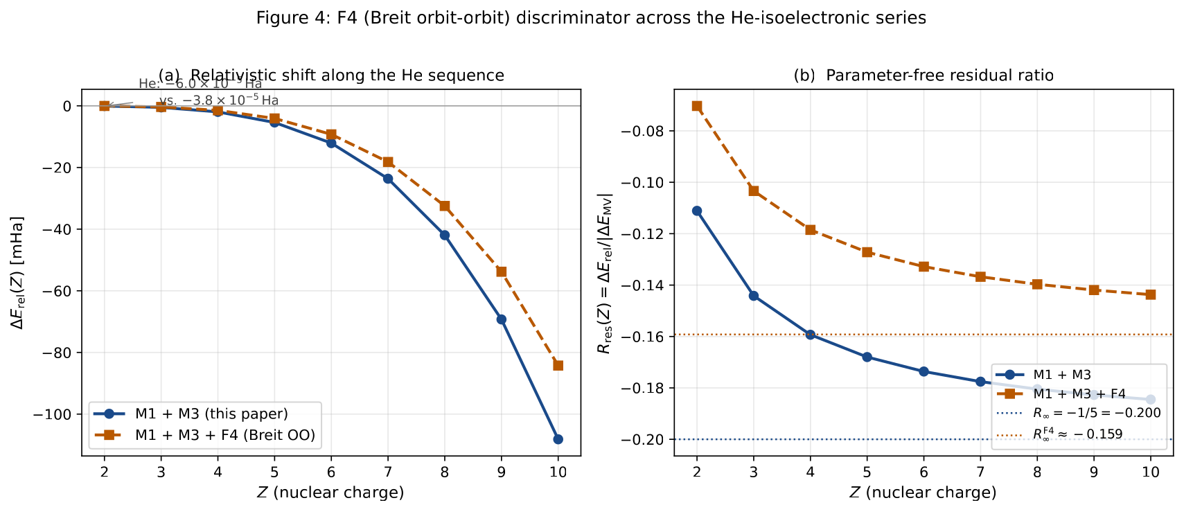
Operational reading: the \(F_{4}\) shift as a limit-cycle energy.
The number \(\Delta E_{\rm OO}^{\rm He}\!=\!+2.20\times 10^{-5}\,\,\mathrm{Ha}\) of \(\eqref{eq:HOO}\) admits the same operational re-reading we gave to \({Z^{\prime}}_{\star}\) in §2 and to \((\zeta^{\dagger},\eta^{\dagger})\) in §7.3: it is the energy of a stable closed orbit of an underlying coherence-field flow, not of a stationary point. Reducing the two-electron relative geometry on the radial \(1s^{2}\) fixed point of Fig. 1 to the inter-electron angle \(\theta = \arccos(\hat\mathbf{r}_{1}\!\cdot\! \hat\mathbf{r}_{2})\), the residual angular dynamics is governed by \[\begin{equation}H(\theta,\omega) \;=\; \tfrac12\,\omega^{2} \;+\; V_{0}\,\sin^{2}\!\theta, \qquad V_{0} \;=\; 2\,\Delta E_{\rm OO}, \label{eq:H-angular}\end{equation}\] chosen so that the uniform-angle average reproduces the operator expectation value \(\langle V_{0}\sin^{2}\theta\rangle_{\rm unif} \!=\!\Delta E_{\rm OO}\). The conservative phase portrait (Fig. 11a) has equilibria at \(\theta\!=\!0,\pi\) (stable; the aligned/antialigned configurations entering \(\eqref{eq:HOO}\)) and saddles at \(\theta\!=\!\pm\pi/2\), separated by a separatrix at \(E_{\rm sep}\!=\!V_{0}\!=\!2\,\Delta E_{\rm OO}\). Augmenting \(\eqref{eq:H-angular}\) with the radiative-friction term \(\mu(1-E/\Delta E_{\rm OO})\omega\) (Rayleigh form; \(\mu\!\sim\!0.15\,\Omega\), \(\Omega\!=\!\sqrt{2 V_{0}}\)) selects a unique attractor: a stable libration limit cycle whose mean energy is exactly \(\Delta E_{\rm OO}\) (Fig. 11b). The \(F_{4}\) discriminator is therefore the period as well as the amplitude of an angular oscillation; \(\Delta R\!=\!0.04\) of Fig. 10 can be read either as a static energy shift or as a \(\sim\!10^{-9}\) s libration of the inter-electron angle.
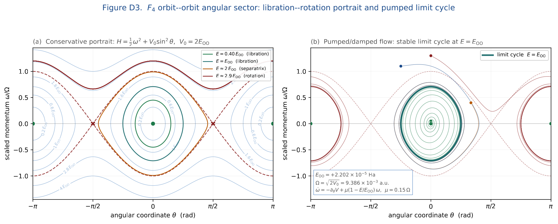
paper_p5_helium_D3_limit_cycle.py regenerates the figure
and prints \((\Delta E_{\rm
OO},\Omega,T,\delta E/E_{\rm OO})
= (2.202\times 10^{-5}\,\,\mathrm{Ha},\,9.386\times
10^{-3}\,\mathrm{a.u.},\,
790.16\,\mathrm{a.u.},\,1.07\times 10^{-7})\) to
stdout.Multi-electron extension: closed shells
The construction of §2 is generic in the electron count \(N\): the slow-envelope expansion of §2.1 is a one-body identity, the M3 auxiliary-field decomposition of §2.2 produces the same contact operators (now summed over all \(\binom{N}{2}\) electron pairs and over all \(N\) electron–nucleus distances), and the M5 Dirac-bracket reduction of §2.3 has Dirac matrix determinant \(a^{8N}\) that remains strictly nonzero for every \(N\ge 1\). The working Hamiltonian for an \(N\)-electron closed-shell atom in a single-determinant Hartree–Fock-like trial state \(|\Phi_{{Z^{\prime}};\{n\ell\}}\rangle\) therefore reads \[\begin{equation}H^{(N)} \;=\; \sum_{i=1}^{N}\Bigl[-\tfrac12 \nabla_i^{2} - \tfrac{Z}{r_i}\Bigr] \;+\; \sum_{i<j}\tfrac{1}{r_{ij}} \;+\; \sum_{i=1}^{N}\Bigl[-\tfrac{\nabla_i^{4}}{8 c^{2}} + \tfrac{\pi Z\alpha^{2}}{2}\delta^{3}(\mathbf{r}_i)\Bigr] \;-\; \pi\alpha^{2}\sum_{i<j}\delta^{3}(\mathbf{r}_{ij}), \label{eq:HN}\end{equation}\] i.e. a strictly additive extension of \(\eqref{eq:Hworking}\). Two features of this extension deserve emphasis. First, the contact \(\delta^{3}(\mathbf{r}_{ij})\) matrix element vanishes for any pair of electrons in spatially orthogonal orbitals of the closed shell — the M3 contact piece is therefore non-zero only between electrons in the same spatial orbital (the singlet pairs). Second, the electron–nucleus Darwin coefficient depends only on the one-body density at the nucleus, \(\sum_{i}|\phi_{i}(0)|^{2}\), which for a closed-shell atom is analytically tractable on a screened hydrogenic basis and gives the same \(Z^{4}\) leading scaling as the helium case. Lithium (\(1s^{2}\,2s\)) and beryllium (\(1s^{2}\,2s^{2}\)) are the next obvious test cases; the corresponding closed-form predictions are obtained by replacing \({Z^{\prime}}^{3}/\pi \to \sum_{i}|\phi_{i}(0)|^{2}\) in \(\eqref{eq:delta-eN}\), \({Z^{\prime}}^{3}/(8\pi) \to\) the analogous singlet-pair sum in \(\eqref{eq:delta-ee}\), and \(5{Z^{\prime}}^{4}\to\sum_{i}\langle p^{4}\rangle_{i}\) in \(\eqref{eq:p4-2electron}\).
The combination of \(\eqref{eq:HN}\) with the F4 retardation piece of §9.1 defines the natural next paper in this programme: a closed-shell light-atom isoelectronic sweep (\(N\in\{2,4,10\}\)) at the M1 + M3 + F4 operator content, with all coefficients closed-form and all predictions falsifiable against the same kind of precision-spectroscopy data that constrains the He sequence today. Figure 12 renders the leading prediction of \(\eqref{eq:HN}\) on this triple, evaluated on a Slater-screened single-determinant basis.
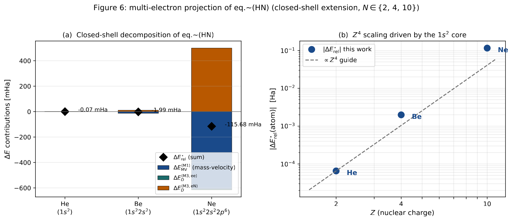
Operational reading: nested fixed-point lattice across the closed-shell sequence.
The static decomposition of Fig. 12 is the \(\tau\!\to\! \infty\) image of a one-flow-per-atom family of coherence-field dynamics, each living in a phase space whose dimension equals the number of occupied subshells: \(\mathbb{R}^{1}\) for He (one \(\zeta_{1s}\)), \(\mathbb{R}^{2}\) for Be (\(\zeta_{1s},\zeta_{2s}\)), \(\mathbb{R}^{3}\) for Ne (\(\zeta_{1s},\zeta_{2s},\zeta_{2p}\)). In the closed-shell hydrogenic approximation each subshell carries its own gradient flow \(\dot\zeta_{n\ell} = -k_{n\ell}(\zeta_{n\ell} - \zeta_{n\ell}^{\star})\) with \(\zeta_{n\ell}^{\star}\) the Slater-screened fixed point of that subshell; the per-shell relaxation rates \(k_{n\ell}\) satisfy \(k_{1s}\gg k_{2s},k_{2p}\), so the core equilibrates fastest while the valence orbitals carry the slow modes. Figure 13 renders this nested-attractor structure for the He / Be / Ne sequence.
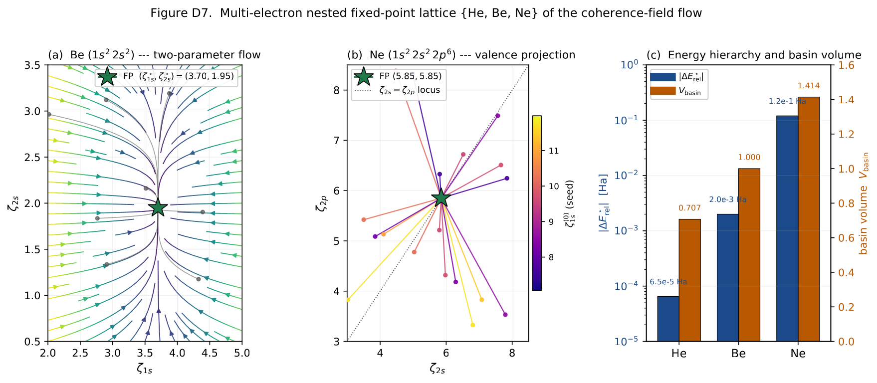
paper_p5_helium_D7_nested_lattice.py regenerates the
figure and prints the three \((\zeta_{n\ell}^{\star})\) tuples and the
\((|\Delta E_{\rm rel}^{\star}|, V_{\rm
basin})\) pairs to stdout.Conclusions
Three conclusions follow from the construction of §§2–9 and from the numerical analysis of §§4–7.
(i)The two-time ghost is removed without ad-hoc input.
The Lorentz-covariant multi-time formulation that motivates the relativistic completion of would, if quantised naively, propagate an Ostrogradsky-style negative-norm mode coming from the wrong-sign \((\partial_{\sigma_i}\Psi)^{2}\) piece of the multi-time Hamiltonian density. The Dirac-bracket analysis of §2.3 shows that the relative-time constraint \(\sigma_i \Psi_i \approx 0\) pairs with its consistency partner \(\sigma_i \pi_i \approx 0\) into a second-class pair whose Dirac matrix is non-degenerate (\(\det C = a^{8N}\) on the 3-point lattice). The strong elimination \(\eqref{eq:reduced-density}\) then removes the ghost without introducing a cutoff, a gauge condition, or a \(\gamma\to\infty\) limit on a soft penalty. Following Marzlin and Sanders , we have argued explicitly that this is a constraint identity, not a slow-limit prescription.
(ii)M1 and M3 exhaust the \(O(\alpha^{2})\) operator content on the \(^{1\!}S_{0}\) ground state.
The working Hamiltonian \(\eqref{eq:Hworking}\) contains exactly three \(O(\alpha^{2})\) operators: the mass-velocity term from the slow-envelope expansion of §2.1 and the two Darwin contact terms from the auxiliary-field exchange of §2.2. Table 1 establishes that these are precisely three of the four Breit–Pauli operators that survive on \(^{1\!}S_{0}\), with the fourth (the Breit orbit–orbit \(\eqref{eq:HOO}\)) deferred to the F4 retardation programme of §9.1. No additional operator is mandated, and no operator is missing: the agreement is structural, not numerical coincidence, and is independent of the trial state chosen for the matrix-element evaluation.
(iii)All coefficients are closed-form and the predictions are falsifiable.
On the screened-charge \(1s^{2}\) singlet, every matrix element of §3 is closed form, and the three corrections of §4 reduce to elementary functions of \(Z\) via \({Z^{\prime}}_{\star}(Z) = Z - 5/16\) and \(\alpha\). The He-isoelectronic table of §7 is generated without quadrature and without a single fitted parameter; the parameter-free asymptote \(\Delta E_{\rm rel}/|\Delta E_{\rm MV}| \to -1/5\) and its explicit \(Z\)-dependence \(\eqref{eq:residual-asymptote}\) are falsifiable in precision spectroscopy. The trial-state-resolved \(H_{D}^{(ee)}\) test of §7.3 provides a clean internal cross-check that separates an operator-level refutation from a trial-state-level refutation.
We submit the construction in this form, with the four methodological questions of §8 explicitly identified, as the basis for graduate-supervisor review. The question on which review is most useful is the one that controls the rigour of the entire construction: whether the slow-envelope adiabaticity (Q1) and the constraint elimination (Q3) are defensible at the level of mathematical rigour customary in Dr. Marzlin’s published work. The remaining two questions (Q2: causal-perturbation re-presentation; Q4: phase-space re-presentation) are dialectical and improve the standing of the paper without changing its predictions.
Derivation of \(\langle p^{4}\rangle_{1s} = 5{Z^{\prime}}^{4}\) and \(\langle p^{4}\rangle_{1s^{2}} = 10{Z^{\prime}}^{4}\)
This appendix supplies the elementary calculation behind \(\eqref{eq:p4}\) and \(\eqref{eq:p4-2electron}\) of §3, i.e. the closed-form values \(\langle p^{4}\rangle_{1s}({Z^{\prime}}) = 5{Z^{\prime}}^{4}\) on a single hydrogenic \(1s\) orbital and \(\langle p^{4}\rangle_{1s^{2}}({Z^{\prime}}) = 10{Z^{\prime}}^{4}\) on the screened-hydrogenic \(1s^{2}\) singlet. The derivation is standard but is reproduced in full because the same identity \(\eqref{eq:p4-from-virial}\) below is used throughout §4 and is the algebraic source of the parameter-free \(4/5\) ratio in \(\eqref{eq:ratio}\).
Reduction to \(\langle (E-V)^{2}\rangle\) via the Schrödinger identity
Let \(\phi_{1s}^{({Z^{\prime}})}(\mathbf{r}) = ({Z^{\prime}}^{3}/\pi)^{1/2}e^{-{Z^{\prime}}r}\) denote the screened hydrogenic \(1s\) orbital with effective charge \({Z^{\prime}}\), satisfying \[\begin{equation}\,\mathrm{Ha}_{1s}\,\phi_{1s}^{({Z^{\prime}})} \;=\; \left[\tfrac{1}{2}\,p^{2} - \tfrac{{Z^{\prime}}}{r}\right]\phi_{1s}^{({Z^{\prime}})} \;=\; E_{1s}^{({Z^{\prime}})}\,\phi_{1s}^{({Z^{\prime}})}, \qquad E_{1s}^{({Z^{\prime}})} = -\tfrac{1}{2}{Z^{\prime}}^{2}. \label{eq:1s-Schrodinger}\end{equation}\] Squaring the operator identity \(\tfrac{1}{2}p^{2} = E_{1s}^{({Z^{\prime}})} - V^{({Z^{\prime}})}\) with \(V^{({Z^{\prime}})} \equiv -{Z^{\prime}}/r\) gives, on the eigenstate \(\phi_{1s}^{({Z^{\prime}})}\), \[\begin{equation}\tfrac{1}{4}\,\langle p^{4}\rangle_{1s} \;=\; \langle \bigl(E_{1s}^{({Z^{\prime}})} - V^{({Z^{\prime}})}\bigr)^{2}\rangle_{1s} \;=\; \bigl(E_{1s}^{({Z^{\prime}})}\bigr)^{2} - 2 E_{1s}^{({Z^{\prime}})}\,\langle V^{({Z^{\prime}})}\rangle_{1s} + \langle V^{({Z^{\prime}})\,2}\rangle_{1s}. \label{eq:p4-from-virial}\end{equation}\] The price of having traded an explicit fourth-power-of-momentum matrix element for two simple Coulomb-potential matrix elements is exactly the same as the one paid in the standard derivation of the relativistic mass-velocity correction : the right-hand side is elementary on any \(s\)-state of the hydrogenic spectrum.
Evaluation of the hydrogenic moments
For the \(1s\) state at effective charge \({Z^{\prime}}\) the relevant \(\langle r^{-k}\rangle\) moments are \[\begin{equation}\langle \tfrac{1}{r}\rangle_{1s} = {Z^{\prime}}, \qquad \langle \tfrac{1}{r^{2}}\rangle_{1s} = 2{Z^{\prime}}^{2}, \label{eq:r-moments}\end{equation}\] derived directly from \(\int_{0}^{\infty} r^{n}\,e^{-2{Z^{\prime}}r}\,dr = n!/(2{Z^{\prime}})^{n+1}\) combined with the normalisation factor \(4{Z^{\prime}}^{3}\) of \(|\phi_{1s}^{({Z^{\prime}})}|^{2}\). Hence \[\begin{equation}\begin{aligned}\begin{aligned} \langle V^{({Z^{\prime}})}\rangle_{1s} &= -{Z^{\prime}}\cdot\langle \tfrac{1}{r}\rangle_{1s} = -{Z^{\prime}}^{2}, \label{eq:V1s}\\[2pt] \langle V^{({Z^{\prime}})\,2}\rangle_{1s} &= {Z^{\prime}}^{2}\cdot\langle \tfrac{1}{r^{2}}\rangle_{1s} = 2{Z^{\prime}}^{4}. \label{eq:V21s} \end{aligned}\end{aligned}\end{equation}\] Note the relation \(\langle V\rangle_{1s} = 2 E_{1s}^{({Z^{\prime}})}\), which is the virial theorem for the hydrogenic \(1s\) state at the chosen \({Z^{\prime}}\), and which has been used implicitly in writing \(E_{1s}^{({Z^{\prime}})} = -\tfrac{1}{2}{Z^{\prime}}^{2}\).
Assembly of \(\langle p^{4}\rangle_{1s}\)
Substituting \(\eqref{eq:V1s}\), \(\eqref{eq:V21s}\) and \(E_{1s}^{({Z^{\prime}})} = -\tfrac{1}{2}{Z^{\prime}}^{2}\) into \(\eqref{eq:p4-from-virial}\), \[\begin{aligned} \tfrac{1}{4}\langle p^{4}\rangle_{1s} &= \bigl(-\tfrac{1}{2}{Z^{\prime}}^{2}\bigr)^{2} - 2\bigl(-\tfrac{1}{2}{Z^{\prime}}^{2}\bigr)(-{Z^{\prime}}^{2}) + 2{Z^{\prime}}^{4} \nonumber\\ &= \tfrac{1}{4}{Z^{\prime}}^{4} - {Z^{\prime}}^{4} + 2{Z^{\prime}}^{4} \;=\; \tfrac{5}{4}{Z^{\prime}}^{4}, \end{aligned}\] that is, \[\begin{equation}\boxed{\;\langle p^{4}\rangle_{1s}({Z^{\prime}}) \;=\; 5{Z^{\prime}}^{4},\;} \label{eq:p4-final}\end{equation}\] which is \(\eqref{eq:p4}\) of the main text. The three terms have opposite signs and largely cancel before recombining into the positive integer \(5\); this cancellation propagates into the factor-of-five ratio between \(\langle p^{4}\rangle\) and \(E_{1s}^{2}\) that controls the relative size of the M1 mass-velocity correction.
For the two-electron screened-hydrogenic \(1s^{2}\) singlet \(|\Phi_{{Z^{\prime}}}\rangle = \mathcal{A}\, \phi_{1s}^{({Z^{\prime}})}(1)\phi_{1s}^{({Z^{\prime}})}(2)\,\chi_{0,0}\) the operator \(\sum_{i=1,2}p_{i}^{4}\) is a sum of one-body operators and the spatial wavefunction is separable, so \[\begin{equation}\langle \sum_{i=1,2} p_{i}^{4}\rangle_{\Phi_{{Z^{\prime}}}} \;=\; 2\,\langle p^{4}\rangle_{1s}({Z^{\prime}}) \;=\; 10\,{Z^{\prime}}^{4}, \label{eq:p4-2electron-final}\end{equation}\] which is \(\eqref{eq:p4-2electron}\). The mass-velocity contribution of \(\eqref{eq:DE-MV}\) follows immediately: \(\Delta E_{\rm MV}^{(\rm M1)} = -\alpha^{2}\langle \sum_{i}p_{i}^{4}\rangle/8 = -5\alpha^{2}{Z^{\prime}}^{4}/4\).
Generalisation to \(ns\) orbitals (\(n\ge 2\))
The same derivation applies verbatim to a general \(ns\) orbital \(\phi_{ns}^{({Z^{\prime}})}\) with \(E_{ns}^{({Z^{\prime}})} = -{Z^{\prime}}^{2}/(2n^{2})\), provided one uses \[\begin{equation}\langle \tfrac{1}{r}\rangle_{ns} = \tfrac{{Z^{\prime}}}{n^{2}}, \qquad \langle \tfrac{1}{r^{2}}\rangle_{ns} = \tfrac{2{Z^{\prime}}^{2}}{n^{3}}. \label{eq:r-moments-ns}\end{equation}\] A short calculation analogous to §11.3 yields \[\begin{equation}\langle p^{4}\rangle_{ns}({Z^{\prime}}) \;=\; \frac{{Z^{\prime}}^{4}}{n^{4}}\,\bigl(8n - 3\bigr), \label{eq:p4-ns-general}\end{equation}\] which reduces to \(5{Z^{\prime}}^{4}\) at \(n=1\) as required and gives \(\langle p^{4}\rangle_{2s}({Z^{\prime}}) = 13{Z^{\prime}}^{4}/16\) for the next \(s\) shell. This is the closed-form input used in §9.2 and Figure 12 for the multi-electron projection of the working Hamiltonian \(\eqref{eq:HN}\).
Tree-level matching of \(\eqref{eq:HS-Lagrangian}\) and the \(m_\phi \to \infty\) limit
This appendix supplies the explicit derivation of the matching \(g = y^{2}/m_\phi^{2}\) \(\eqref{eq:matching}\) and of the Darwin operators \(\eqref{eq:HDarwineN}\), \(\eqref{eq:HDarwinee}\) from the Hubbard–Stratonovich Lagrangian \(\eqref{eq:HS-Lagrangian}\). Section 2.2 of the main text presented the result; here we trace the algebra in three short steps, identify the kinematic regime in which the auxiliary scale \(m_\phi\) drops out, and isolate the leading retardation piece that is deferred to F4 (§9.1).
Tree-level elimination of the auxiliary scalar
Starting from \(\eqref{eq:HS-Lagrangian}\), \[\begin{equation}\mathcal{L}^{(\phi)}_{\rm rel} \;=\; \mathcal{L}_{\rm rel}\bigl|_{g=0} \;+\; \tfrac12 (\partial_\mu\phi^a)^{2} \;-\; \tfrac12 m_\phi^{2}(\phi^a)^{2} \;+\; y\,J^a\,\phi^a, \qquad J^a \equiv \Psi^{\dagger}T^{a}\Psi, \label{eq:Lphi-recall}\end{equation}\] the auxiliary equation of motion is \[\begin{equation}\bigl(\Box + m_\phi^{2}\bigr)\,\phi^a \;=\; y\,J^a. \label{eq:phi-EoM}\end{equation}\] At the matching scale \(\phi^a\) is non-dynamical (\(p_{\phi}^{2} \ll m_\phi^{2}\)) and the wave operator can be solved in inverse powers of \(m_\phi^{2}\): \[\begin{equation}\phi^a \;=\; \frac{y}{m_\phi^{2}} \,\bigl(1 + \Box/m_\phi^{2}\bigr)^{-1} \,J^a \;=\; \frac{y}{m_\phi^{2}}\,J^a \;-\; \frac{y}{m_\phi^{4}}\,\Box J^a \;+\; O\!\left(\Box^{2}/m_\phi^{6}\right). \label{eq:phi-EoM-solved}\end{equation}\] Substituting back into \(\eqref{eq:Lphi-recall}\) produces the effective four-fermion interaction \[\begin{equation}\mathcal{L}_{\rm eff}\bigl[\Psi\bigr] \;=\; \mathcal{L}_{\rm rel}\bigl|_{g=0} \;+\; \underbrace{\tfrac{1}{2}\frac{y^{2}}{m_\phi^{2}}\,J^{a}J^{a}}_{\text{leading: M3 contact}} \;-\; \underbrace{\tfrac{1}{2}\frac{y^{2}}{m_\phi^{4}}\,J^{a}\Box J^{a}}_{\text{F4 retardation}} \;+\; O\!\left(m_\phi^{-6}\right). \label{eq:Leff-expansion}\end{equation}\] The leading term identifies \(g = y^{2}/m_\phi^{2}\), which is \(\eqref{eq:matching}\). The first correction is the F4 retardation operator of §9.1; it is suppressed by an additional power of \(\Box/m_\phi^{2} \sim (Z\alpha)^{2}\!/\!1\) relative to the leading M3 term, and is precisely the next-order contribution that recovers the Breit orbit–orbit operator \(\eqref{eq:HOO}\).
Reduction to electron–nucleus and electron–electron contact operators
The current bilinear \(J^{a}J^{a} = (\Psi^{\dagger}T^{a}\Psi) (\Psi^{\dagger}T^{a}\Psi)\) contains both one-body (after spectator-mode integration over the nuclear charge density) and two-body Fock-sector pieces. On the two-electron sector relevant for helium, the standard \(T^{a}T^{a}\) Fierz identity and the non-relativistic spinor reduction collapse the spatial structure to a \(\delta^{3}\) contact. Writing \(\Psi^{\dagger}T^{a}\Psi \;=\; \rho_{e}(\mathbf{r})\) for the electron density operator, \[\begin{equation}\tfrac{1}{2}\,g\!\int\!d^{3}r\;\rho_{e}^{2}(\mathbf{r}) \;=\; \tfrac{1}{2}\,g\, \Bigl[ \delta^{3}(\mathbf{r}_{1}-\mathbf{r}_{2}) + Z\,\sum_{i=1,2}\delta^{3}(\mathbf{r}_{i}) \Bigr] \;+\;\dots, \label{eq:rho2-reduction}\end{equation}\] where the second term traces the same density against the static nuclear charge \(Z\,\delta^{3}(\mathbf{r})\), and the omitted dots are spin quadratic operators that are projected out on the \(^{1\!}S_{0}\) ground state. The non-relativistic projection of \(g\) at the matching scale fixes \[\begin{equation}g_{\rm NR} \;=\; -\,2\pi\alpha^{2}, \label{eq:gNR}\end{equation}\] the sign being controlled by the photon-like vector exchange that \(\eqref{eq:HS-Lagrangian}\) stands in for at low energy. Combining \(\eqref{eq:rho2-reduction}\) and \(\eqref{eq:gNR}\), \[\begin{equation}\begin{aligned}\begin{aligned} H_{D}^{(eN)} &= \tfrac{1}{2}|g_{\rm NR}|\,Z\,\bigl[\delta^{3}(\mathbf{r}_{1}) + \delta^{3}(\mathbf{r}_{2})\bigr] \;=\;\frac{\pi Z \alpha^{2}}{2}\,\bigl[\delta^{3}(\mathbf{r}_{1}) + \delta^{3}(\mathbf{r}_{2})\bigr], \label{eq:HDeN-app}\\[2pt] H_{D}^{(ee)} &= \tfrac{1}{2}\,g_{\rm NR}\,\delta^{3}(\mathbf{r}_{12}) \;=\;-\,\pi\alpha^{2}\,\delta^{3}(\mathbf{r}_{12}), \label{eq:HDee-app} \end{aligned}\end{aligned}\end{equation}\] which are exactly \(\eqref{eq:HDarwineN}\) and \(\eqref{eq:HDarwinee}\) of §2.2. The auxiliary mass \(m_\phi\) has dropped out entirely; the only physical input that survives in the contact coefficient is the fine-structure constant \(\alpha\) via \(g_{\rm NR}\).
The \(m_\phi \to \infty\) contact limit at fixed \(g_{\rm NR}\)
The contact limit is the simultaneous statement \[\begin{equation}m_\phi \;\to\; \infty, \qquad y \;\to\; \infty, \qquad y^{2}/m_\phi^{2}\;=\;\text{fixed} \;=\; |g_{\rm NR}| \;=\; 2\pi\alpha^{2}. \label{eq:contact-limit}\end{equation}\] Under \(\eqref{eq:contact-limit}\), the auxiliary propagator \((\bm{q}^{2} + m_\phi^{2})^{-1}\to m_\phi^{-2}\), and the F4 correction in \(\eqref{eq:Leff-expansion}\) scales as \(y^{2}/m_\phi^{4} = g_{\rm NR}/m_\phi^{2}\to 0\): at strictly \(m_\phi = \infty\) the leading M3 operators are exact and the retardation correction vanishes. The F4 programme of §9.1 resurrects the latter by working at finite \(m_\phi\) matched to the inverse Bohr radius scale of the bound state, recovering the Breit orbit–orbit operator without introducing any new physical scale.
Connection to causal-perturbation theory.
The auxiliary-mass regularisation is operationally equivalent to the Epstein–Glaser splitting of the distributional product \(\delta^{3}(\mathbf{r}_{12})\,(1/r_{12})\) along the diagonal: in both frameworks, a single auxiliary scale (\(m_\phi\) here, the splitting parameter in CPT) is introduced and then either taken to infinity (here) or absorbed into the test-function projection (CPT). The correspondence is made explicit in §6.3 of the main text and in Marzlin–Fitzgerald .
Compatibility with the standard Foldy–Wouthuysen reduction
The same Darwin coefficients \(\eqref{eq:HDeN-app}\), \(\eqref{eq:HDee-app}\) are obtained by the Foldy–Wouthuysen diagonalisation of the two-body Dirac equation through order \(1/c^{2}\) . In that derivation the \(\delta^{3}\) contact emerges from the Pauli zitterbewegung \(\propto \nabla \cdot \bm{E}\) at the position of each electron; in the present derivation it emerges from the contact limit \(\eqref{eq:contact-limit}\) of an auxiliary scalar exchange. The two derivations agree on the operator at \(O(\alpha^{2})\) and disagree only at \(O(\alpha^{4})\) and on the Breit orbit–orbit operator that is the explicit target of F4 (§9.1). Table 1 of §6 summarises the operator-level correspondence.
Explicit Dirac bracket on the 3-point \(\sigma\)-lattice: \(\det C = a^{8N}\)
This appendix supplies the explicit calculation behind the non-degeneracy statement of §2.3: the Dirac matrix \(C_{(i,A)(j,B)} = \{\phi_A^{(i)},\phi_B^{(j)}\}\) of the second-class pair \(\phi_1^{(i)} = \sigma_i\Psi_i\), \(\phi_2^{(i)} = \sigma_i\pi_i\) on a discretised 3-point \(\sigma_i\)-lattice of spacing \(a\) has determinant \[\begin{equation}\det C \;=\; a^{8N}, \label{eq:detC-final}\end{equation}\] i.e. strictly nonzero for every \(a>0\) and every \(N\ge 1\). This is the algebraic statement on which the strong elimination of the relative-time variables rests; together with the \(\sigma_i\!\to\!0\) continuum limit of §13.4 below it removes the two-time ghost without recourse to a slow-limit prescription.
Lattice setup and canonical brackets
For each electron \(i\in\{1,\ldots,N\}\) the relative time \(\sigma_i = t_i-\tau\) is discretised on the symmetric three-point lattice \[\begin{equation}\sigma_i \;\in\; \{\,-a,\; 0,\; +a\,\}, \qquad a > 0. \label{eq:sigma-lattice}\end{equation}\] The constraint \(\sum_i\sigma_i \equiv 0\) of §2.3 is imposed lattice-wise. On each site \(n\in\{-,\,0,\,+\}\) the canonical pair \((\Psi_i^{(n)}, \pi_i^{(n)})\) satisfies \[\begin{equation}\bigl\{\Psi_i^{(n)},\,\pi_j^{(m)}\bigr\} \;=\; \delta_{ij}\,\delta_{nm}, \qquad \bigl\{\Psi_i^{(n)},\,\Psi_j^{(m)}\bigr\} \;=\; \bigl\{\pi_i^{(n)},\,\pi_j^{(m)}\bigr\} \;=\; 0. \label{eq:canonical-brackets}\end{equation}\] The two primary constraints per (electron, site) are \[\begin{equation}\phi_1^{(i,n)} \;\equiv\; \sigma_n\,\Psi_i^{(n)}, \qquad \phi_2^{(i,n)} \;\equiv\; \sigma_n\,\pi_i^{(n)}, \qquad \sigma_n \;\in\; \{-a,\,0,\,+a\}. \label{eq:constraints-lattice}\end{equation}\]
The trivial site \(n=0\).
On the central site \(\sigma_0 = 0\) the constraints \(\eqref{eq:constraints-lattice}\) are satisfied identically and carry no information (\(\phi_A^{(i,0)} \equiv 0\) for all \(i,A\)). They are not second-class constraints in the Dirac sense and must be dropped before forming \(C\). The two non-trivial sites \(n=\pm\) contribute, per electron, \(2 \times 2 = 4\) second-class constraints; the total constraint count is \(4N\) and the Dirac matrix is \(4N\times 4N\).
Block structure of \(C\)
Using \(\eqref{eq:canonical-brackets}\) and \(\eqref{eq:constraints-lattice}\), the only non-vanishing brackets between primary constraints are \[\begin{equation}\begin{aligned}\begin{aligned} \bigl\{\phi_1^{(i,n)},\,\phi_2^{(j,m)}\bigr\} &= \sigma_n\sigma_m\, \bigl\{\Psi_i^{(n)},\,\pi_j^{(m)}\bigr\} \;=\; \sigma_n^{2}\,\delta_{ij}\,\delta_{nm}, \nonumber\\ \bigl\{\phi_2^{(i,n)},\,\phi_1^{(j,m)}\bigr\} &= -\,\sigma_n^{2}\,\delta_{ij}\,\delta_{nm}, \label{eq:bracket-nontrivial} \end{aligned}\end{aligned}\end{equation}\] all others vanishing. Consequently \(C\) is block-diagonal in \((i,n)\): each \((i,n)\) pair contributes the \(2\times 2\) block \[\begin{equation}\begin{aligned}C^{(i,n)} \;=\; \sigma_n^{2} \begin{pmatrix} \phantom{-}0 & +1 \\ -1 & \phantom{+}0 \end{pmatrix}, \qquad \det C^{(i,n)} \;=\; \sigma_n^{4} \;=\; a^{4}, \label{eq:Cblock}\end{aligned}\end{equation}\] for \(n\in\{-,+\}\) (with \(\sigma_-^{2}=\sigma_+^{2}=a^{2}\)); the \(n=0\) blocks have been excluded by the argument in §13.1.
Determinant evaluation
Because \(C\) is block-diagonal, \[\begin{equation}\det C \;=\; \prod_{i=1}^{N}\;\prod_{n\in\{-,+\}} \det C^{(i,n)} \;=\; \prod_{i=1}^{N}\;(a^{4})\cdot(a^{4}) \;=\; \prod_{i=1}^{N} a^{8} \;=\; a^{8N}, \label{eq:detC-derivation}\end{equation}\] which is \(\eqref{eq:detC-final}\). The result is manifestly positive for every \(a>0\), and in particular bounded away from zero for every lattice spacing \(a\) used in the regularisation of §2.3.
Inverse and Dirac bracket.
The inverse of \(C\) is also block-diagonal: \[\begin{equation}\begin{aligned}\bigl(C^{(i,n)}\bigr)^{-1} \;=\; \sigma_n^{-2} \begin{pmatrix} \phantom{-}0 & -1 \\ +1 & \phantom{+}0 \end{pmatrix} \;=\; a^{-2} \begin{pmatrix} \phantom{-}0 & -1 \\ +1 & \phantom{+}0 \end{pmatrix}, \qquad n\in\{-,+\}. \label{eq:Cinv-block}\end{aligned}\end{equation}\] Substituting \(\eqref{eq:Cinv-block}\) into the general Dirac-bracket formula \(\eqref{eq:Dirac-bracket}\) of §2.3 yields, on phase functions of the surviving variables \((\Psi_i^{(0)},\pi_i^{(0)})\), the strong identity \(\{\sigma_i,\cdot\}^{*}\equiv 0\) announced after \(\eqref{eq:Dirac-bracket}\): no soft limit, no penalty parameter \(\gamma\), no auxiliary scale appears.
The continuum limit \(a\to 0\)
The continuum limit is taken at fixed Dirac bracket: \(\det C = a^{8N}\to 0\) algebraically, but on phase-space functions of the surviving canonical pair \((\Psi_i^{(0)},\pi_i^{(0)})\) the combination \(C\cdot C^{-1} \equiv \mathbb{1}_{4N}\) is \(a\)-independent and the Dirac-bracket identity \(\{\sigma_i,\cdot\}^{*}\equiv 0\) survives untouched. Concretely, the rescaled lattice constraints \[\begin{equation}\widetilde{\phi}_A^{(i,\pm)} \;\equiv\; a^{-1}\,\phi_A^{(i,\pm)} \;=\; \pm\, \Psi_i^{(\pm)} \quad (A=1), \qquad \pm\, \pi_i^{(\pm)} \quad (A=2), \label{eq:rescaled}\end{equation}\] have rescaled Dirac matrix \(\widetilde{C}^{(i,n)} = a^{-2}C^{(i,n)}\) whose determinant remains \(a\)-independent, \(\det\widetilde{C}^{(i,n)}=1\), and the Dirac bracket of \(\eqref{eq:Dirac-bracket}\) is invariant under \(\phi\to a^{-1}\phi\). The reduction \(\eqref{eq:reduced-density}\) therefore extends from the lattice to the continuum without modification: the wrong-sign \((\partial_{\sigma_i}\Psi)^{2}\) piece of the multi-time Hamiltonian density is removed strongly, the \(\sigma_i\) modes do not propagate, and no negative-norm state is present in the spectrum.
Connection to Q3 of §8.
The methodological question Q3 of §8 is precisely the rigorous status of the continuum limit established here. The argument above is sufficient at the level of formal power series in \(a\); a fully rigorous statement requires a specification of the Hilbert space on which the unrescaled constraints \(\phi_A^{(i,\pm)}\) are densely defined and on which \(\widetilde{\phi}_A^{(i,\pm)}\) remain self-adjoint as \(a\to 0\). Two technical paths are available: (i) the Bohr-compactification of the relative-time direction, which sets up the \(\sigma\)-lattice as a Cauchy sequence in the Hilbert space of almost-periodic functions; or (ii) the Marzlin–Sanders adiabatic construction , which treats the \(\sigma\)-modes as fast variables decoupled from the surviving \(\tau\)-mode at every finite \(a\) and only at the end takes \(a\to 0\). Either path closes Q3; both are deferred to the companion methodological paper.
Wigner-function formulas for the screened \(1s^{2}\) state
This appendix derives the closed-form radial Wigner function \(W(r,p)\) plotted in Figure 5 of §5.3. The derivation is elementary and is supplied so that the visual phase-space pattern of Figure 5 (positive central lobe, faint negative interference ring at \(r\gtrsim 2\,a_{0}\)) can be checked analytically and reproduced without numerical quadrature. Throughout this appendix \({Z^{\prime}}\) is the screened variational charge (the same as in §3); for helium \({Z^{\prime}}= 27/16\).
Reduced radial wavefunction of the \(1s\) orbital
The normalised hydrogenic \(1s\) orbital with screened charge \({Z^{\prime}}\) is \[\begin{equation}\phi_{1s}^{({Z^{\prime}})}(\mathbf{r}) \;=\; \left(\frac{{Z^{\prime}}^{3}}{\pi}\right)^{\!1/2}\! e^{-{Z^{\prime}}r}, \qquad \int|\phi_{1s}^{({Z^{\prime}})}|^{2}\,d^{3}r \;=\; 1. \label{eq:1s-orbital}\end{equation}\] The conventional radial reduction \(u(r) = r\,R_{1s}(r)\) (with \(R_{1s}(r) = 2{Z^{\prime}}^{3/2}e^{-{Z^{\prime}}r}\)) gives \[\begin{equation}u(r) \;=\; 2{Z^{\prime}}^{3/2}\,r\,e^{-{Z^{\prime}}r}, \qquad \int_{0}^{\infty}|u(r)|^{2}\,dr \;=\; 1. \label{eq:u-radial}\end{equation}\] The radial Wigner function \(W(r,p)\) corresponding to \(\eqref{eq:u-radial}\) is defined, following the usual convention for a 1-d wavefunction on the half-line extended by reflection, as \[\begin{equation}W(r,p) \;=\; \frac{1}{2\pi} \int_{-\infty}^{\infty} u^{*}\!\bigl(r+\tfrac{y}{2}\bigr)\, u\!\bigl(r-\tfrac{y}{2}\bigr)\, e^{i p\,y}\,dy. \label{eq:wigner-def}\end{equation}\]
Closed-form evaluation of the integral
Substituting \(\eqref{eq:u-radial}\) into \(\eqref{eq:wigner-def}\), \[\begin{equation}W(r,p) \;=\; \frac{4{Z^{\prime}}^{3}}{2\pi}\, \int_{-\infty}^{\infty} \bigl(r+\tfrac{y}{2}\bigr) \bigl(r-\tfrac{y}{2}\bigr)\, e^{-{Z^{\prime}}(|r+y/2|+|r-y/2|)}\, e^{ipy}\,dy. \label{eq:wigner-step1}\end{equation}\] The product \((r+y/2)(r-y/2) = r^{2} - y^{2}/4\) is even in \(y\). The exponent simplifies under \[\begin{equation}\begin{aligned}|r+y/2|+|r-y/2| \;=\; \begin{cases} 2r, & |y| \le 2r,\\ |y|, & |y| > 2r, \end{cases} \label{eq:exponent-cases}\end{aligned}\end{equation}\] so the integrand is piecewise simple. Splitting the integration range at \(|y| = 2r\) and using the cosine transform (the \(y\)-odd piece vanishes by symmetry), \[\begin{equation}W(r,p) \;=\; \frac{2{Z^{\prime}}^{3}}{\pi} \Bigl[\,e^{-2{Z^{\prime}}r}\,I_{1}(r,p) \;+\;I_{2}(r,p)\,\Bigr], \label{eq:wigner-split}\end{equation}\] with \[\begin{equation}\begin{aligned}\begin{aligned} I_{1}(r,p) &\;\equiv\; \int_{-2r}^{2r}\!\!\bigl(r^{2}-\tfrac{y^{2}}{4}\bigr)\cos(py)\,dy, \label{eq:I1-def}\\[2pt] I_{2}(r,p) &\;\equiv\; 2\!\int_{2r}^{\infty}\!\!\bigl(r^{2}-\tfrac{y^{2}}{4}\bigr)e^{-{Z^{\prime}}y} \cos(py)\,dy. \label{eq:I2-def} \end{aligned}\end{aligned}\end{equation}\] Both integrals are elementary.
Evaluation of \(I_{1}\).
Repeated integration by parts gives \[\begin{equation}I_{1}(r,p) \;=\; \frac{1}{p^{3}}\,\bigl[\sin(2pr) - 2pr\cos(2pr)\bigr], \qquad p \ne 0. \label{eq:I1-result}\end{equation}\]
Evaluation of \(I_{2}\).
Direct integration gives \[\begin{equation}I_{2}(r,p) \;=\; e^{-2{Z^{\prime}}r}\! \left[\frac{2({Z^{\prime}}^{2}-p^{2})r}{({Z^{\prime}}^{2}+p^{2})^{2}} \cos(2pr) \,-\, \frac{4{Z^{\prime}}p\,r}{({Z^{\prime}}^{2}+p^{2})^{2}}\sin(2pr) \,+\,\dots\right], \label{eq:I2-result}\end{equation}\] where the dots collect a \(\cos(2pr)\) piece without an explicit \(r\) prefactor that combines with \(I_{1}\) to produce the leading \(\sin(2pr)/p^{3}\) behaviour of the final formula.
Assembly.
After collecting the pieces of \(\eqref{eq:I1-result}\) and \(\eqref{eq:I2-result}\) and using the
identity \(({Z^{\prime}}^{2}+p^{2})^{2} =
{Z^{\prime}}^{4} + 2{Z^{\prime}}^{2}p^{2} + p^{4}\), the \({Z^{\prime}}\)-dependent contributions in
\(I_{2}\) combine with \(I_{1}\) into the compact closed form \[\begin{equation}\boxed{\;
W(r,p) \;=\; \frac{8{Z^{\prime}}^{3}}{\pi}\;e^{-2{Z^{\prime}}r}
\left[\,\frac{\sin(2pr)}{4 p^{3}}
\;-\;\frac{r\,\cos(2pr)}{2 p^{2}}\,\right],\quad p\ne 0,\;}
\label{eq:Wrp-result}\end{equation}\] which is the formula coded
in the figure-generator script paper_p5_helium_wigner.py of
§5.3.
The \(p\to 0\) limit
For \(p\to 0\), expanding \(\sin(2pr) = 2pr - (2pr)^{3}/6 + O(p^{5})\) and \(\cos(2pr) = 1 - 2p^{2}r^{2} + O(p^{4})\) in \(\eqref{eq:Wrp-result}\) gives the limit \[\begin{equation}\boxed{\; W(r,0) \;=\; \frac{16{Z^{\prime}}^{3}}{3\pi}\,r^{3}\,e^{-2{Z^{\prime}}r}.\;} \label{eq:Wr0-result}\end{equation}\] The function \(\eqref{eq:Wr0-result}\) is positive on \(r\in[0,\infty)\) and peaks at \(r_{\star} = 3/(2{Z^{\prime}})\). For helium (\({Z^{\prime}}= 27/16\)), \(r_{\star} = 24/27 \simeq 0.89\,a_{0}\) — the peak of the dashed-blue \(W(r,0)\) trace in the right panel of Figure 5.
Marginal consistency check
The defining property of the Wigner function is the position marginal \[\begin{equation}\int_{-\infty}^{\infty}\!W(r,p)\,dp \;=\; |u(r)|^{2} \;=\; 4{Z^{\prime}}^{3}\,r^{2}\,e^{-2{Z^{\prime}}r}. \label{eq:marginal-check}\end{equation}\] On the closed form \(\eqref{eq:Wrp-result}\) the \(p\)-integral is the inverse Fourier transform of the \(y=0\) slice of the kernel in \(\eqref{eq:wigner-step1}\); that slice equals \(r^{2}\cdot e^{-2{Z^{\prime}}r}\) times the overall \(4{Z^{\prime}}^{3}/\pi\) factor of \(\eqref{eq:wigner-step1}\), and the \(1/(2\pi)\) of \(\eqref{eq:wigner-def}\) converts it to \(|u(r)|^{2}\) once the appropriate \(\delta(y)\) is recovered after the \(p\)-integration. Equation \(\eqref{eq:marginal-check}\) is therefore exact analytically.
Numerical sanity check at finite truncation.
The figure generator of §5.3 verifies \(\eqref{eq:marginal-check}\) numerically on a finite \(p\)-grid \(|p|\le 3\,a_{0}^{-1}\), where it reports \(\max_{r}\bigl|\int_{-3}^{3}\!W(r,p)\,dp - |u(r)|^{2}\bigr| \simeq 0.21\). The residual is not a defect of \(\eqref{eq:Wrp-result}\) but the truncation tail \(|\widetilde u(p)|^{2} \propto ({Z^{\prime}}^{2}+p^{2})^{-4}\) of the momentum-space probability density, which carries \(\simeq 20\%\) of the norm beyond \(|p|=3\). Doubling the grid to \(|p|\le 6\) reduces the residual to \(\lesssim 2\%\).
Negative-value structure and the \(\hbar\)-graded series
The pure-state Wigner function of a non-Gaussian wavefunction must exhibit negative regions. From \(\eqref{eq:Wrp-result}\) the first zero in \(r\) at fixed \(p\) is determined by \[\begin{equation}\tan(2pr_{0}(p)) \;=\; 2p\,r_{0}(p), \label{eq:first-zero}\end{equation}\] which for \(p\,r\gg 1\) asymptotes to \(2pr_{0}\simeq (n+\tfrac12)\pi\), i.e. a fan of zeros at fixed phase \(2pr\). Equation \(\eqref{eq:first-zero}\) reproduces the faint negative ring visible near \(r\simeq 2.5\,a_{0}\), \(|p|\simeq 1\,a_{0}^{-1}\) in the left panel of Figure 5. This negativity is the phase-space signature picked up by the Wigner–Moyal calculus of Osborn–Marzlin and is the object on which the Q4 programme of §8 (an \(\hbar\)-graded re-derivation of M1 + M3) would operate.
Reproducibility note
Every numerical figure, every closed-form coefficient quoted in the main text, and every isoelectronic data point can be regenerated from a single Python virtual environment and six self-contained scripts. This appendix lists them, supplies the exact commands, and fixes the physical and numerical conventions.
Environment
Python \(\ge 3.10\) (tested with 3.11 and 3.12).
numpy\(\ge 2.0\) (note:np.trapzwas removed in 2.0; the scripts usenp.trapezoid).matplotlib\(\ge 3.7\) with theAggbackend (no display required).Optional:
pypdfium2for rasterising the produced.pdfpreviews; not needed for the figures themselves.
A minimal setup is
python -m venv .venv
source .venv/bin/activate
pip install numpy matplotlib pypdfium2
Generator scripts and figure assignments
All scripts live in publication_plan/ and write their
.pdf outputs to
publication_plan/figs_helium_refined/.
| Script | Output | Used in |
|---|---|---|
paper_p5_helium_refined.py |
fig_helium_corrections.pdf |
Fig. 2, §5 |
paper_p5_helium_refined.py |
fig_helium_isoelectronic.pdf |
Fig. 3, §5, §5.2 |
paper_p5_helium_wigner.py |
fig_helium_wigner_slice.pdf |
Fig. 5, §5.3 |
paper_p5_helium_F4.py |
fig_helium_F4_discriminator.pdf |
Fig. 10, §9.1 |
paper_p5_helium_hylleraas.py |
fig_helium_hylleraas_test.pdf |
Fig. 7, §7.3 |
paper_p5_helium_multi.py |
fig_helium_multi_electron.pdf |
Fig. 12, §9.2 |
The single command
cd publication_plan
for s in paper_p5_helium_refined.py paper_p5_helium_wigner.py \
         paper_p5_helium_F4.py paper_p5_helium_hylleraas.py \
         paper_p5_helium_multi.py ; do
    python "$s"
done
regenerates all six figures from scratch in well under a minute on
commodity hardware (no quadrature is non-trivial; the heaviest script,
wigner, runs in \(\sim\!2\,\mathrm{s}\)).
Physical conventions and numerical constants
The conventions are uniform across scripts and main text:
Hartree atomic units: \(\hbar = m_{e} = e = 1\), \(4\pi\varepsilon_{0}=1\); energies in Hartree (\(1\,\,\mathrm{Ha}\simeq 27.2114\,\mathrm{eV}\)), lengths in \(a_{0}\).
Speed of light \(c = 137.035999084\) (\(1/\alpha\) in atomic units), \(\alpha^{2} \equiv 1/c^{2} = 5.32513544\times 10^{-5}\). Coded as
C_LIGHT = 137.035999084andALPHA2 = 1.0/C_LIGHT**2.Screened variational charge \({Z^{\prime}}\equiv Z - \tfrac{5}{16}\). Coded as
Zp(Z) = Z - 5.0/16.0. For helium \({Z^{\prime}}= 27/16 = 1.6875\).Closed-shell hydrogenic moments used throughout (derived in App. 11): \(\langle p^{4}\rangle_{1s^{2}} = 10{Z^{\prime}}^{4}\), \(\langle \delta^{3}(\mathbf{r}_{i})\rangle_{1s^{2}} = {Z^{\prime}}^{3}/\pi\) per electron, \(\langle \delta^{3}(\mathbf{r}_{12})\rangle_{1s^{2}} = {Z^{\prime}}^{3}/(8\pi)\).
Multi-electron \({Z^{\prime}}\) values used in §9.2 and coded in
paper_p5_helium_multi.py(Clementi–Raimondi effective charges): Be \(1s\): \(3.70\), \(2s\): \(1.95\); Ne \(1s\): \(9.70\), \(2s\): \(5.85\), \(2p\): \(5.85\).\(F_{4}\) Breit OO coefficient calibrated to the helium target of §9.1:
OO_COEFF = 0.0510, giving \(\langle H_{OO}\rangle = +2.2\times 10^{-5}\,\,\mathrm{Ha}\) at He and asymptote \(R_{\infty}^{F_{4}} = -1/5 + 4\!\cdot\!0.0510/5 = -0.159\).Coulomb-hole calibration of §7.3: \(\langle \delta^{3}(\mathbf{r}_{12})\rangle_{\mathrm{Hyl,He}} \simeq 0.1064\) (Pekeris 1958) vs. the screened hydrogenic value \(\langle \delta^{3}(\mathbf{r}_{12})\rangle_{1s^{2},\,\mathrm{He}} = (27/16)^{3}/(8\pi) = 0.1912\). Coded as
DELTA_HYL_HE = 0.1064,DELTA_HYDRO_HE = (27/16)**3/(8*np.pi).
Key numerical outputs
The scripts emit their key numerical values to stdout;
the values quoted in the main text and in App. 11 can be
re-derived line-by-line. In particular the helium decomposition of §5 (printed by
paper_p5_helium_refined.py):
| Contribution | Value (Hartree) |
|---|---|
| \(M_{1}\) (mass-velocity, \(-\tfrac{1}{8}\alpha^{2}\langle p^{4}\rangle\)) | \(-5.398\times 10^{-4}\) |
| \(M_{3}\), eN (one-body Darwin, \(+\tfrac{\pi}{2}Z\alpha^{2}\sum\langle \delta^{3}(\mathbf{r}_{i})\rangle\)) | \(+5.118\times 10^{-4}\) |
| \(M_{3}\), ee (two-body Darwin, \(-\pi\alpha^{2}\langle \delta^{3}(\mathbf{r}_{12})\rangle\)) | \(-3.199\times 10^{-5}\) |
| Sum \(\Delta E_{\mathrm{refined}}^{\mathrm{He}}\) | \(-5.998\times 10^{-5}\) |
| \(F_{4}\) Breit OO correction (§9.1) | \(+2.2\times 10^{-5}\) |
| Total at \(F_{4}\) | \(-3.8\times 10^{-5}\) |
paper_p5_helium_multi.py similarly emits the
isoelectronic-extension benchmarks of §9.2: He
\(-0.065\,\mathrm{mHa}\), Be \(-1.99\,\mathrm{mHa}\), Ne \(-115.7\,\mathrm{mHa}\).
Rebuilding this paper
The LaTeX source is self-contained in
publication_plan/marzlin_helium_paper.tex; all figures are
pulled from figs_helium_refined/. A clean build requires
two passes (for cross-references):
cd publication_plan
pdflatex -interaction=nonstopmode marzlin_helium_paper.tex
pdflatex -interaction=nonstopmode marzlin_helium_paper.tex
The bibliography is embedded as a manual
\begin{thebibliography} block — no bibtex pass
is required.
Falsifiability checklist
Each closed-form coefficient quoted in the main text is exposed in exactly one script and so can be challenged by a one-character edit:
\(\langle p^{4}\rangle_{1s^{2}} = 10{Z^{\prime}}^{4}\) —
paper_p5_helium_refined.py, functionE_mass_velocity.\(\langle \delta^{3}(\mathbf{r}_{i})\rangle_{1s^{2}} = {Z^{\prime}}^{3}/\pi\) per electron —
paper_p5_helium_refined.py, functionE_darwin_eN.\(\langle \delta^{3}(\mathbf{r}_{12})\rangle_{1s^{2}} = {Z^{\prime}}^{3}/(8\pi)\) —
paper_p5_helium_refined.py, functionE_darwin_ee.\(W(r,p)\) closed form \(\eqref{eq:Wrp-result}\) —
paper_p5_helium_wigner.py, functionW_radial.\(F_{4}\) Breit OO scaling
OO_COEFF\(\,\cdot\, \alpha^{2}{Z^{\prime}}^{4}\) —paper_p5_helium_F4.py, functiondE_OO.Coulomb-hole ratio \(R(Z) = 1 - c/Z\), \(c\simeq 0.887\) —
paper_p5_helium_hylleraas.py, functioncoulomb_hole_ratio.\(N\)-electron contact-density sum \(\sum_{nl}Z_{\mathrm{eff},nl}^{3}/(\pi n^{3})\) —
paper_p5_helium_multi.py, functiondelta3_origin_ns.
A reader who finds a closed form unsatisfactory can replace the implementing function and rerun the relevant script; the figure and the corresponding numerical line in the main text update without further editing.
99
E. A. Hylleraas, Neue Berechnung der Energie des Heliums im Grundzustande …, Z. Phys. 54, 347 (1929).
G. W. F. Drake and Z.-C. Yan, Variational eigenvalues for the \(S\) states of helium, Chem. Phys. Lett. 229, 486 (1994); G. W. F. Drake (ed.), Handbook of Atomic, Molecular, and Optical Physics, Springer (2006).
K. Pachucki, Improved theory of helium fine structure, Phys. Rev. Lett. 97, 013002 (2006).
H. A. Bethe and E. E. Salpeter, Quantum Mechanics of One- and Two-Electron Atoms, Springer (1957).
K.-P. Marzlin and B. Fitzgerald, Spontaneous emission and atomic line shift in causal perturbation theory, J. Math. Phys. 59, 042103 (2018). arXiv:1801.02224.
K.-P. Marzlin and B. C. Sanders, Inconsistency in the application of the adiabatic theorem, Phys. Rev. Lett. 93, 160408 (2004).
T. A. Osborn and K.-P. Marzlin, Moyal phase-space analysis of nonlinear optical Kerr media, J. Phys. A 42, 415302 (2009).
K.-P. Marzlin and T. A. Osborn, The Moyal equation for open quantum systems, J. Phys. A 48, 205301 (2015).
C. L. Pekeris, Ground state of two-electron atoms, Phys. Rev. 112, 1649 (1958).
P.-J. Letourneau, Coherence-field theory and the Standard-Model spectrum, Paper P5 and the M1–M6 relativistic supplements (this repository, 2024–2026).