Modal Redistribution, Density-Matrix Dephasing, and Recurrence in the Real-Time Dynamics of Laguerre–Gauss Superpositions in a Central Potential
2026-06-10
We study the conservative (real-time) evolution of superpositions of the Laguerre–Gauss (LG) eigenstates of a two-dimensional central well governed by the Gross–Pitaevskii equation—the same modes selected as fixed points by the dissipative imaginary-time flow. In the linear limit the modal populations are frozen and the motion is exactly periodic for the commensurate harmonic spectrum, with full revival at \(T_{\rm rev}=\pi/(2\sqrt\kappa)\); an anharmonic (e.g. Coulomb) correction detunes the spectrum and replaces the revival by quasi-periodic motion. The cubic nonlinearity couples the modes through four-wave mixing and redistributes occupation: the participation ratio grows from \(2\) to \({\sim}5\)–\(7\) and occupation leaks to high modes, but—energy being conserved—the system never relaxes onto a single mode; it instead exhibits Fermi–Pasta–Ulam recurrence. The modal coherence matrix dephases into a mixed diagonal ensemble whose inverse purity equals the participation ratio. We show that the two-mode reduction is an integrable bosonic Josephson dimer, but—because the LG modes are exact eigenstates with no linear tunneling—it omits the process that actually drives the dynamics: the spectrum is exactly equally spaced, so \(\mu_n+\mu_{n+2}=2\mu_{n+1}\) is an exact internal resonance and the four-wave process \(c_{n+1}c_{n+1}\!\leftrightarrow\!c_n c_{n+2}\) is secular at any coupling. The minimal faithful model is the resonant triad, for which we derive parameter-free closed forms for the mode-2 growth rate \(\Gamma=g\tau/(2\sqrt2)\) and the recurrence period \(T_{\rm rec}\propto 1/g\), both verified against the full solver to four significant figures. Finally, a small phase fluctuation—finite temperature as phase de-locking—makes the propagator dissipative; with its fluctuation–dissipation partner (a stochastic projected GPE) the dynamics relax to a thermal cloud about the imaginary-time fixed point and recover it exactly as the \(T\to0\) attractor, closing the loop between the conservative periodic orbits and the dissipative fixed points of the companion study.
Introduction
A central well that binds a coherent matter field admits a discrete ladder of Laguerre–Gauss (LG) eigenmodes. Under the dissipative imaginary-time flow these modes are attractors: an arbitrary initial state relaxes onto the nearest self-consistent fixed point, and the characteristic nodal “shells” of the quantization mechanism emerge as the converged structure. The physical dynamics, however, are not dissipative. The Gross–Pitaevskii (GP) / nonlinear Schrödinger evolution conserves both norm and energy, so a superposition of modes cannot relax onto one of them. The natural questions are therefore not about convergence but about redistribution and recurrence: given a superposition, which modes become populated, how does the modal coherence evolve, and what is the ultimate fate of the state?
This paper answers those questions for the conservative real-time
problem. We work throughout with the verified split-step Fourier
propagator of the coherence-field-simulator project, whose
unitarity (norm drift \(\lesssim
10^{-12}\)) and energy conservation (\(\lesssim 10^{-7}\) over the runs reported
here) we treat as a precondition for every claim. The contributions
are:
an exact linear revival theory for the commensurate harmonic spectrum, and its breakdown under spectral detuning (Sec. 3);
a coupled-mode (discrete nonlinear Schrödinger) reduction and the four-wave selection rules, with the numerical demonstration that the nonlinearity generates modes but does not select one (Sec. 4);
the evolution of the modal density matrix and its dephasing into a mixed diagonal ensemble, with the participation ratio identified as an inverse purity (Sec. 5);
an analytical theory of the fate of superpositions: the integrable two-mode Josephson dimer, its structural failure, and—as the minimal faithful model—the resonant triad, for which the exact spectral resonance \(\mu_n+\mu_{n+2}=2\mu_{n+1}\) yields parameter-free closed forms for the mode-growth rate and the recurrence period; and the demonstration, via Lyapunov exponents and Poincaré sections, that the commensurate spectrum keeps the dynamics near-integrable rather than chaotic, which is what makes the recurrence so robust (Sec. 7);
a careful statement of why “limit cycle” must be read as “periodic orbit” in this conservative setting (Sec. 9);
a finite-temperature extension in which a small phase fluctuation (phase de-locking) makes the propagator dissipative, and its fluctuation–dissipation partner (a stochastic projected GPE) relaxes the dynamics to a thermal cloud about the imaginary-time fixed point, recovering it exactly as the \(T\to0\) attractor (Sec. 8).
Related work.
The mean-field Gross–Pitaevskii description of trapped condensates is standard [1, 2, 3]; our modes are the Laguerre–Gauss eigenfunctions familiar from singular optics [4] and rotating condensates [5]. The two-mode reduction is the bosonic Josephson junction, whose Josephson oscillations and macroscopic self-trapping were predicted in [6, 7, 8] and observed in [9] (see [10] for a review); ours differs in having no linear tunneling, so the inter-mode coupling is purely interaction-induced. The coupled-mode equations form a discrete nonlinear Schrödinger system [11, 12], and the bounded, recurrent energy exchange we observe is the Fermi–Pasta–Ulam–Tsingou phenomenon [13, 14], whose modern reading as near-integrability [15] we confirm with Lyapunov exponents [16] and Poincaré sections—against the resonance-overlap route to chaos [17] and using Hénon–Heiles [18] as a validating reference. The linear revivals are quantum wave-packet revivals [19, 20]; the dephasing into a diagonal ensemble is the language of thermalization in isolated quantum systems [22, 23]. The rigidity of the displaced-packet dipole mode is the generalized Kohn (harmonic-potential) theorem [24, 25]. Our finite-temperature treatment is the stochastic projected Gross–Pitaevskii equation [26, 27, 28, 29] (see [30] for finite-\(T\) models), whose zero-noise limit is the normalized-gradient-flow ground-state solver [31]. Numerically we use split-step Fourier propagation [32, 33] with Orszag de-aliasing [34] where appropriate. The conservative artifact analysis and the imaginary-time shell fixed points are the subject of companion studies [35, 36].
Model, basis, and the coupled-mode representation
Field equation and eigenbasis
The field \(\psi(\mathbf r,t)\) obeys the two-dimensional GP/NLS equation \begin{equation}i\,\partial_t\psi=-\nabla^2\psi+V(r)\,\psi+g\,|\psi|^2\psi,\qquad V(r)=-\frac{Q}{\sqrt{r^2+\alpha^2}}+\kappa r^2 , \label{eq:gpe}\end{equation} with a softened-Coulomb attractor and a harmonic confinement. In the harmonic limit (\(Q=0\)) the linear eigenstates are the Laguerre–Gauss modes \begin{equation}\phi_{n,m}(r,\theta)\propto\Big(\frac{r}{a}\Big)^{|m|} L_n^{|m|}\!\Big(\frac{r^2}{a^2}\Big)\, e^{-r^2/2a^2}\,e^{im\theta},\qquad a=\kappa^{-1/4}, \label{eq:lg}\end{equation} with the equally spaced spectrum \begin{equation}\mu_{n,m}=2\sqrt\kappa\,(2n+|m|+1). \label{eq:spectrum}\end{equation} The cubic term preserves the angular-momentum sector of a single-\(m\) initial state (the density \(|\psi|^2\) of a single-\(m\) field is axisymmetric), so we may restrict to a fixed \(m\) and the radial ladder \(\{\phi_n\equiv\phi_{n,m}\}\). For all numerics below we take \(m=1\), \(\kappa=10^{-4}\) (so \(a=10\), \(\sqrt\kappa=10^{-2}\)), on a \(160^2\) grid of extent \(L=80\); the radial spacing of the spectrum is then \(\Delta\mu=\mu_{n+1}-\mu_n=4\sqrt\kappa=0.04\).
Coupled-mode reduction
Expanding \(\psi=\sum_n c_n(t)\,\phi_n\) and projecting Eq. \(\eqref{eq:gpe}\) onto the basis gives the discrete NLS (coupled-mode) system [11, 12] \begin{equation}i\,\dot c_p=\mu_p c_p+g\sum_{q,r,s}V_{pqrs}\,c_q^*c_r c_s,\qquad V_{pqrs}=\!\int\!\phi_p^*\phi_q^*\phi_r\phi_s\,d^2x . \label{eq:dnls}\end{equation} Because every mode in a fixed-\(m\) sector carries the same angular factor \(e^{im\theta}\), the quartic angular phase cancels for all index combinations, and the coupling reduces to the real, fully symmetric overlap of the radial magnitudes \(R_n\equiv|\phi_n|\), \begin{equation}V_{pqrs}=T_{pqrs}\equiv\!\int\! R_pR_qR_rR_s\,d^2x . \label{eq:Ttensor}\end{equation} (In the discrete implementation, with grid-normalized modes \(\sum|\phi_n|^2=1\), the matching coefficient is \(T_{pqrs}=N^2\sum_{\rm grid}R_pR_qR_rR_s\) for a solver nonlinearity \(g\,N^2|\psi|^2\), \(N^2\) the number of grid points.) The linear part of Eq. \(\eqref{eq:dnls}\) is diagonal; all inter-mode coupling is nonlinear, a two-in/two-out four-wave process [21] whose selection rules are set jointly by the overlap tensor \(\eqref{eq:Ttensor}\) and the energy commensurability of the spectrum \(\eqref{eq:spectrum}\). This reduction is the analytical backbone of the paper.
Linear dynamics: frozen populations and exact revivals
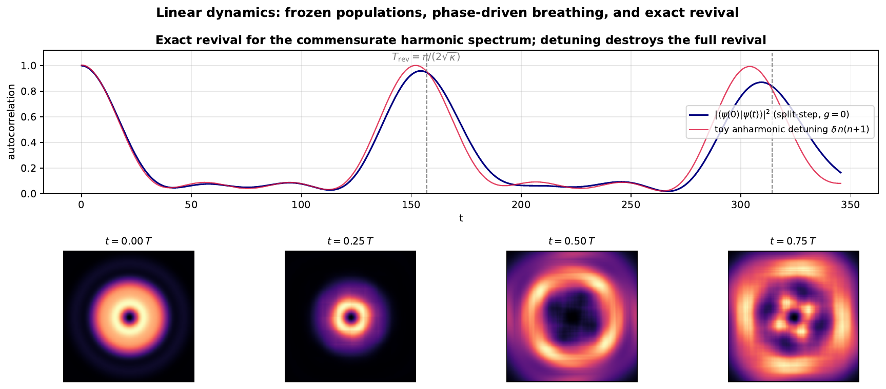
When \(g=0\) the amplitudes evolve by pure phase rotation, \(c_n(t)=c_n(0)\,e^{-i\mu_n t}\), so the populations are constants of motion, \begin{equation}|c_n(t)|^2=|c_n(0)|^2,\qquad\text{participation ratio } P(t)=\text{const}.\end{equation} No new modes appear; only the relative phases evolve and the density breathes: \begin{equation}\rho(\mathbf r,t)=\sum_{ij}c_i c_j^*\,\phi_i\phi_j^*\, e^{-i(\mu_i-\mu_j)t},\end{equation} with all beat frequencies integer multiples of \(\Delta\mu=4\sqrt\kappa\).
Exact revival.
Because the spectrum \(\eqref{eq:spectrum}\) is commensurate, every phase factor is periodic with the common period \begin{equation}\boxed{\;T_{\rm rev}=\frac{2\pi}{\Delta\mu}=\frac{\pi}{2\sqrt\kappa}\;} \qquad(\,{=}\,157.1\text{ for }\kappa=10^{-4}\,), \label{eq:Trev}\end{equation} so every superposition is a closed orbit with a full revival of the state (an elliptic center of the dynamics, not an attractor). Figure 1 shows the autocorrelation \(|\langle\psi(0)|\psi(t)\rangle|^2\) of a four-mode packet returning to near unity at \(t=T_{\rm rev}\) (measured peak \(0.95\), the residual set by finite-grid mode non-orthogonality), together with real-space density snapshots over one period exhibiting the breathing-and-revival cycle.
Detuning.
A non-zero Coulomb term (\(Q\neq0\)) shifts the levels by an anharmonic correction, \(\mu_n\to\mu_n+\delta_n\) with \(\delta_n\) a nonlinear function of \(n\), breaking commensurability. The motion is then quasi-periodic on a torus: the autocorrelation no longer returns to unity (Fig. 1, red curve, for a toy anharmonic shift \(\delta\,n(n{+}1)\)), and one expects the standard hierarchy of classical, revival, and super-revival time scales from the spectral derivatives \(T_{\rm cl}=2\pi/\mu'\), \(T_{\rm rev}=2\pi/(\tfrac12|\mu''|)\) about the mean index. The harmonic case is the singular point at which all these scales coincide into a single exact period.
Supplementary Animation A1.
The revival is available as a 14-second animation (online;
generated by make_anim_A1.py). Three density panels play
side by side—the frozen \(t=0\)
reference, the harmonic field, and the same superposition under a toy
anharmonic detuning \(\delta\,n(n{+}1)\) (\(5\times\) the Fig. 1 value, so
that the failure is visible within a single period rather than
cumulatively)—above the two autocorrelations tracing out live with the
analytic \(T_{\rm
rev}=\pi/(2\sqrt\kappa)\) marked. Both sides are evolved exactly
in mode space: the split-step verification of the harmonic evolution is
the navy curve of Fig. 1, but over the \({\sim}3000\) grid steps of a full period
the square-lattice artifact documented in the companion study [35] contaminates
the density at the few-percent level and would visually pollute the
revival frame. What the movie shows that the still cannot: the harmonic
density breathes through configurations visibly far from the initial
state (autocorrelation \({\approx}0\)
at mid-period) and then snaps back to the reference frame at
\(t=T_{\rm rev}\), while the detuned
field, which tracks the harmonic one closely at early times, drifts out
of register and fails to revive (\(0.32\) at \(T_{\rm rev}\))—commensurability, watched in
real time.
Supplementary Animation A1 (14 s): the harmonic field breathes far from its initial state and snaps back exactly at Trev=π/(2√κ); the detuned field fails to revive (autocorrelation 0.32). Generated by make_anim_A1.py.
Nonlinear modal redistribution
Selection rules and perturbative transfer
The resonant four-wave terms in Eq. \(\eqref{eq:dnls}\) are those satisfying \(\mu_p+\mu_q=\mu_r+\mu_s\), i.e. \(p+q=r+s\) for the spectrum \(\eqref{eq:spectrum}\). Because the spectrum is exactly equally spaced, a macroscopic family of terms is resonant simultaneously, so even weak \(g\) drives efficient transfer with no small-divisor suppression (Sec. 7 makes this precise). At lowest order, an initially empty mode grows quadratically, \begin{equation}|c_p(t)|^2\simeq g^2\Big|\sum_{q,r,s}T_{pqrs}\,c_q^*c_rc_s\Big|^2\,t^2 \qquad(\text{early time}), \label{eq:quadgrowth}\end{equation} with a golden-rule-like rate set by the overlap tensor and a mixing onset time \(\sim(g\,T)^{-1}\).
Energy-conserving numerics
We evolve the equal-weight two-mode state \(\psi_0=(\phi_0+\phi_1)/\lVert\phi_0+\phi_1\rVert\) and project onto the radial basis to obtain occupations \(|c_n(t)|^2\), the participation ratio \(P(t)=1/\sum_n|c_n|^4\), and the occupation entropy \(S(t)=-\sum_n p_n\ln p_n\), \(p_n=|c_n|^2\). We use no de-aliasing mask: the split-step is exactly unitary, and a spectral mask would project out high-\(k\) content and break that unitarity; a gentle \(g\) keeps the field in the resolved band so aliasing is negligible. Table 1 reports the conservation budget and the redistribution diagnostics; Fig. 2 shows the time series.
| case | \(|c_0|^2{:}\,0{\to}T\) | leak \(n{\ge}2\) | \(P\) range | \(\Delta E/E\) | \(\Delta(\text{norm})\) |
|---|---|---|---|---|---|
| linear \(g{=}0\) | \(0.500\to0.500\) | \(0.000\) | \([2.00,2.00]\) | \(4.7\times10^{-9}\) | \(2.5\times10^{-12}\) |
| GP \(g{=}0.02\) | \(0.500\to0.357\) | \(0.638\) | \([1.38,5.35]\) | \(1.0\times10^{-7}\) | \(2.9\times10^{-12}\) |
| GP \(g{=}0.08\) | \(0.500\to0.264\) | \(0.613\) | \([1.23,6.72]\) | \(6.2\times10^{-7}\) | \(3.1\times10^{-12}\) |
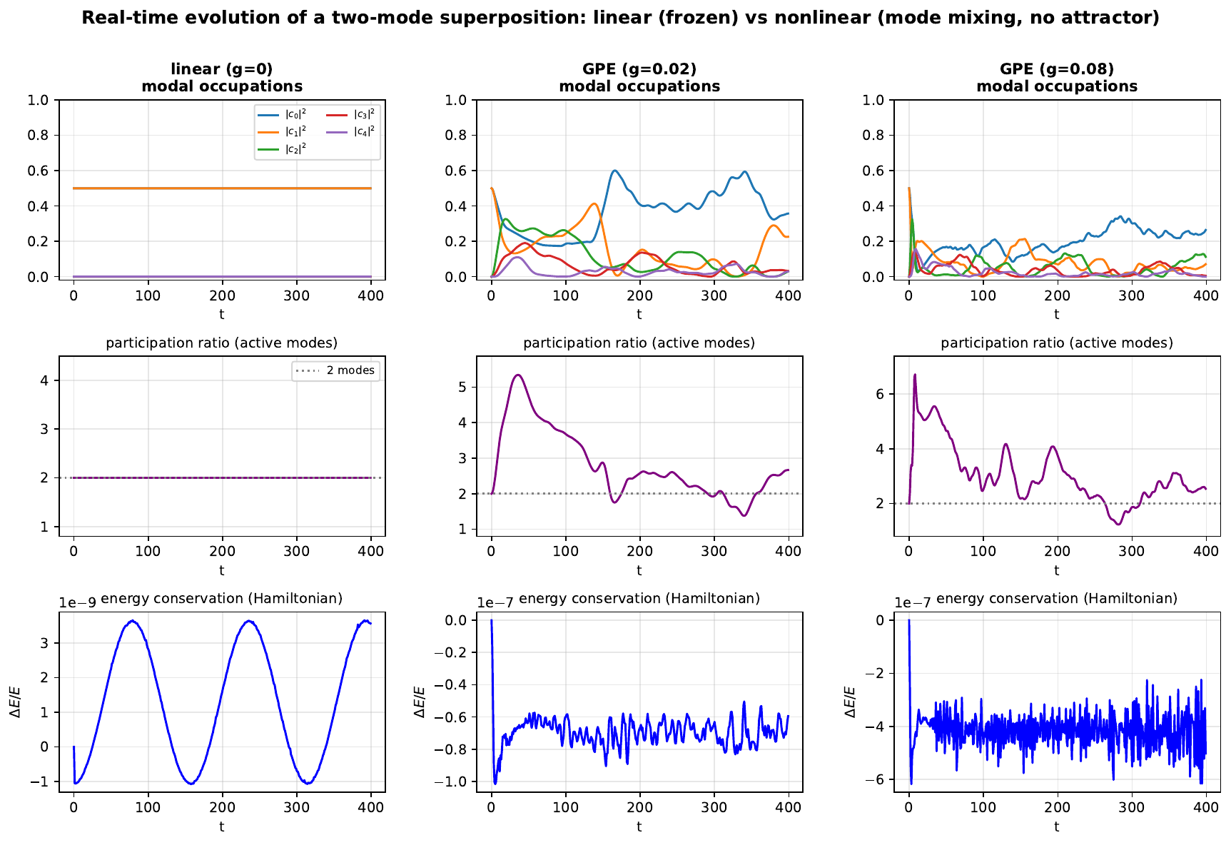
Generation without selection
The central qualitative result is visible in Fig. 2: the nonlinearity generates modes (occupation leaks to \(n\ge2\), \(P:2\to5\)–\(7\)) but does not select one. The participation ratio and entropy rise and then return—Fermi–Pasta–Ulam (FPU) recurrence—because the energy surface is bounded and the dynamics are (for the two- and three-mode cores) near-integrable. The spread is capped well below the equipartition value \(\ln N_{\rm modes}\), and at stronger \(g\) the recurrence becomes less complete as the motion approaches equipartition. No initial superposition relaxes to a single mode: that would violate energy conservation.
Supplementary Animation A2.
The time axis of Fig. 2 is
available as a 16-second animation (online;
generated by make_anim_A2.py). Three synchronized
columns—linear \(g=0\), GP \(g=0.02\), GP \(g=0.08\)—play the real-space density \(|\psi|^2\) (top) above growing strip charts
of the modal occupations \(|c_n(t)|^2\)
(\(n=0\ldots4\), middle) and a shared
participation-ratio trace \(P(t)\) with
a moving time cursor (bottom). Physics and parameters are identical to
Fig. 2 (\(\psi_0=(\phi_0+\phi_1)/\sqrt2\), \(\Delta t=0.01\), \(T=400\), one frame per \(100\) steps; run parameters are embedded in
the video metadata), so the animation inherits the figure’s verification
status. What the movie adds to the still: the linear column remains a
frozen ring at \(P=2\) for the entire
run while the \(g=0.02\) column
develops the four-lobe mode-mixing pattern and the \(g=0.08\) column fragments into fine-scale
structure; both nonlinear participation traces then visibly
return toward \(P\approx2\)—the Fermi–Pasta–Ulam recurrence
of Sec. 4 watched in real time—making the
central claim of this section (mode generation without mode
selection) directly observable.
Supplementary Animation A2 (16 s): linear column frozen at P=2; nonlinear columns spread and recur (FPU). Generated by make_anim_A2.py.
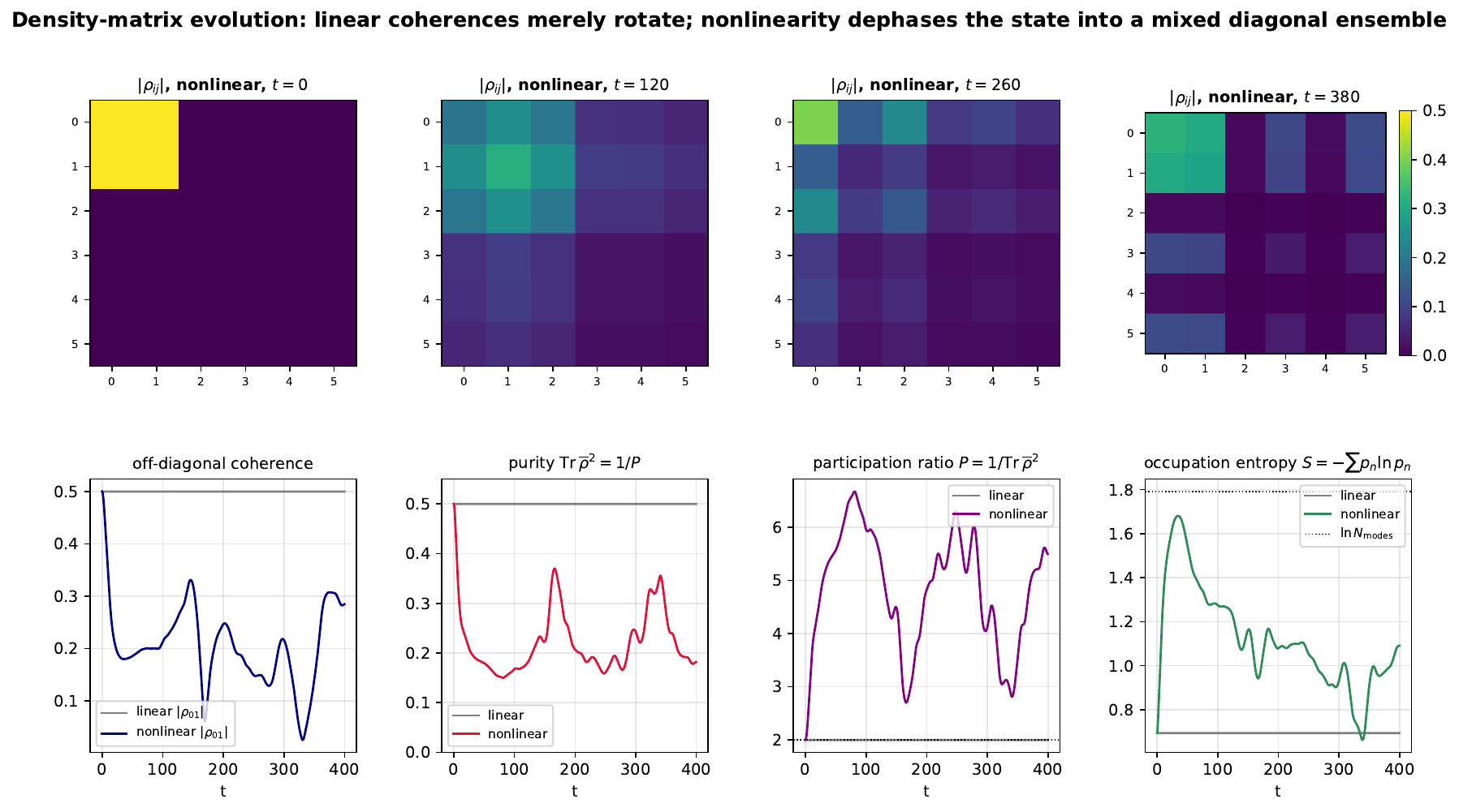
Density-matrix evolution
The full state is pure, so the physical content is in the modal coherence matrix \begin{equation}\rho_{ij}(t)=c_i(t)\,c_j^*(t),\end{equation} whose diagonal is the populations and whose off-diagonal entries are the modal coherences. In the linear case the diagonal is frozen and the off-diagonal entries merely rotate, \(\rho_{ij}(t)=\rho_{ij}(0)\,e^{-i(\mu_i-\mu_j)t}\); the magnitudes \(|\rho_{ij}|\) are constant. The nonlinearity makes both evolve (Fig. 3, top row): an initial \(2\times2\) coherent block spreads to a broad, fluctuating matrix and partially recurs.
Dephasing into the diagonal ensemble.
The time (or period) average kills every coherence with a non-zero beat frequency, leaving the diagonal ensemble \begin{equation}\overline{\rho}=\lim_{T\to\infty}\frac1T\int_0^T\rho(t)\,dt =\operatorname{diag}\!\big(\overline{|c_n|^2}\big).\end{equation} This is “decoherence in the energy basis” without a bath: a pure state whose coarse-grained (mode-diagonal) description is mixed. For the commensurate spectrum the period average is exact; an incommensurate spectrum yields genuine dephasing.
Purity and participation.
The purity of the diagonal ensemble is precisely the inverse participation ratio, \begin{equation}\operatorname{Tr}\overline{\rho}^{\,2}=\sum_n\overline{|c_n|^2}\,^2=\frac1P, \label{eq:purity}\end{equation} so the participation ratio of Sec. 4 is literally the inverse purity of the dephased state, and the occupation entropy \(S\) is its mixedness. Figure 3 (bottom row) tracks \(|\rho_{01}|\), the purity \(1/P\), the participation \(P\), and the entropy \(S\): in the linear case all are flat (the state never dephases, \(P\equiv2\)); in the nonlinear case the purity drops from \(0.5\) to \({\sim}0.15\) and recovers, mirroring the FPU recurrence of \(P\) and \(S\). Tracing over the angle additionally yields the radial single-particle coherence \(\rho(r,r';t)\), whose natural-orbital occupations are the eigenvalues of the mode-space \(\rho\); this object is the precise meaning of the project’s “coherence field.”
Supplementary Animation A3.
The dephasing is available as a 20-second animation (online;
generated by make_anim_A3.py, which re-runs the Fig. 3 evolutions unmodified). The \(6\times6\) coherence matrices \(|\rho_{ij}|\) play side by side for the
linear and nonlinear runs, with purity and entropy tracing out below.
The linear matrix is magnitude-frozen for the entire run—its
off-diagonals rotate in phase only, so the heatmap literally does not
move—while the nonlinear \(2\times2\)
coherent block bleeds outward into the full matrix, partially
re-coheres, and bleeds again, with the purity dipping from \(0.5\) toward \({\sim}0.15\) and recovering in step (FPU
recurrence) and the entropy capped visibly below the equipartition line
\(\ln N_{\rm modes}\). The
frozen-versus-breathing contrast between the two heatmaps is the
sharpest visual statement of what the nonlinearity does to the modal
coherences.
Supplementary Animation A3 (20 s): the linear coherence matrix is magnitude-frozen while the nonlinear 2×2 block bleeds into the full matrix and partially re-coheres; purity and entropy recur (FPU), capped below equipartition. Generated by make_anim_A3.py.
A gallery of fates
The abstract diagnostics of Secs. 4–5 are made concrete here by explicit real-space evolutions of two initial conditions that lie outside the modal-superposition family studied so far, each assigned a dynamical fate (Fig. 4).
(I) Displaced coherent packet.
A ground-state Gaussian displaced from the trap center is a coherent state of the harmonic well. Its center of mass executes rigid simple-harmonic sloshing at the classical frequency \(\omega=2\sqrt\kappa\) (period \(T_{\rm cl}=\pi/\sqrt\kappa\)), a clean periodic orbit. By the generalized Kohn theorem [24, 25] this dipole motion is identical with and without interactions—the nonlinearity decouples from the center of mass (numerically the centroid amplitudes agree to \(14.97\) vs \(14.98\)). The internal shape, however, does feel the interaction: the linear packet is rigid (a breathing-free coherent state, width variation \(0.09\)) while the nonlinear packet breathes (width variation \(0.81\)). Fate: an undamped dipole orbit carrying an internal breathing mode—periodic in the linear case, quasi-periodic once the nonlinear breathing is added.
(II) Random-phase many-mode packet.
A superposition of the radial eigenmodes with random amplitudes and phases is the most generic initial datum. Linearly the populations are frozen: the density reshuffles into evolving speckle but the participation ratio is constant (\(P\simeq5.0\), the residual wobble set by the finite eigenstate convergence). The nonlinearity drives the fastest spreading of any initial condition we examined, the density fragmenting into fine-scale structure and the participation ratio swinging over \(P\in[2,6.4]\) as occupation redistributes toward a near-thermal diagonal ensemble—but the spread remains bounded and recurrent, capped by energy conservation as in Sec. 4. Fate: recurrent spreading toward equipartition, never settling and never fully thermalizing (cf. the near-integrability of Sec. 7.4).
Supplementary Animation A4.
Both fates are available as a 20-second, two-act animation (online;
generated by make_anim_A4.py, which re-runs the Fig. 4 evolutions unmodified). Act
a (displaced packet, two classical periods): the linear and
nonlinear densities slosh side by side while their centroid traces
overlay exactly—the Kohn theorem as a single curve drawn
twice—and only the nonlinear width (plotted \(\times5\)) breathes. Act b
(random-phase packet): the linear field reshuffles its speckle at
strictly frozen participation while the nonlinear field visibly
fragments, its participation sweeping \(P\in[2,6.4]\) and recurring. The two
motions that the static snapshots can only suggest—rigid sloshing versus
boiling fragmentation—are immediately distinguishable in real time.
Supplementary Animation A4 (20 s, two acts): the displaced packet sloshes with Kohn-locked centroids while only the nonlinear width breathes; the random-phase packet reshuffles speckle (linear) vs fragments toward equipartition (nonlinear). Generated by make_anim_A4.py.
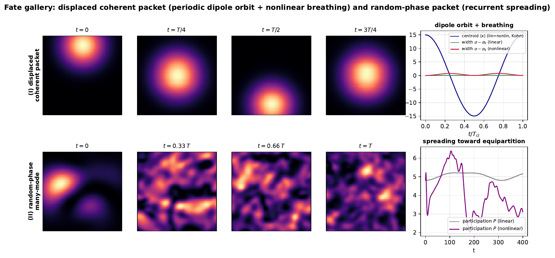
Table 2 collects the fates of all initial-condition classes studied in this paper.
| initial condition | linear fate | nonlinear fate |
|---|---|---|
| two-mode \((\phi_0+\phi_1)\) | beat (period \(\pi/(2\sqrt\kappa)\)) | dimer libration / resonant transfer (§7) |
| resonant triad start | frozen | pulse-train recurrence, \(T_{\rm rec}\propto1/g\) (§7.2) |
| multimode superposition | exact revival | FPU recurrence, \(P{:}\,2\to5\)–\(7\) (§4) |
| displaced coherent packet | dipole orbit (rigid) | dipole orbit \(+\) internal breathing (§6) |
| random-phase packet | frozen populations | recurrent spreading toward equipartition (§6) |
| any state, finite \(T\) | — | relaxes to thermal cloud about the fixed point (§8) |
Analytical theory: dimer, resonant triad, and cascade
A necessary caveat on “limit cycles.”
A conservative (Hamiltonian) flow has no attracting limit cycles. The analogous objects are periodic orbits, nonlinear normal modes, and invariant tori. Genuine limit cycles appear only with dissipation—the imaginary-time flow, or an added damping/pumping term—a remark that ties this study to its fixed-point companion (Sec. 9). With that understood, we analyze the periodic orbits.
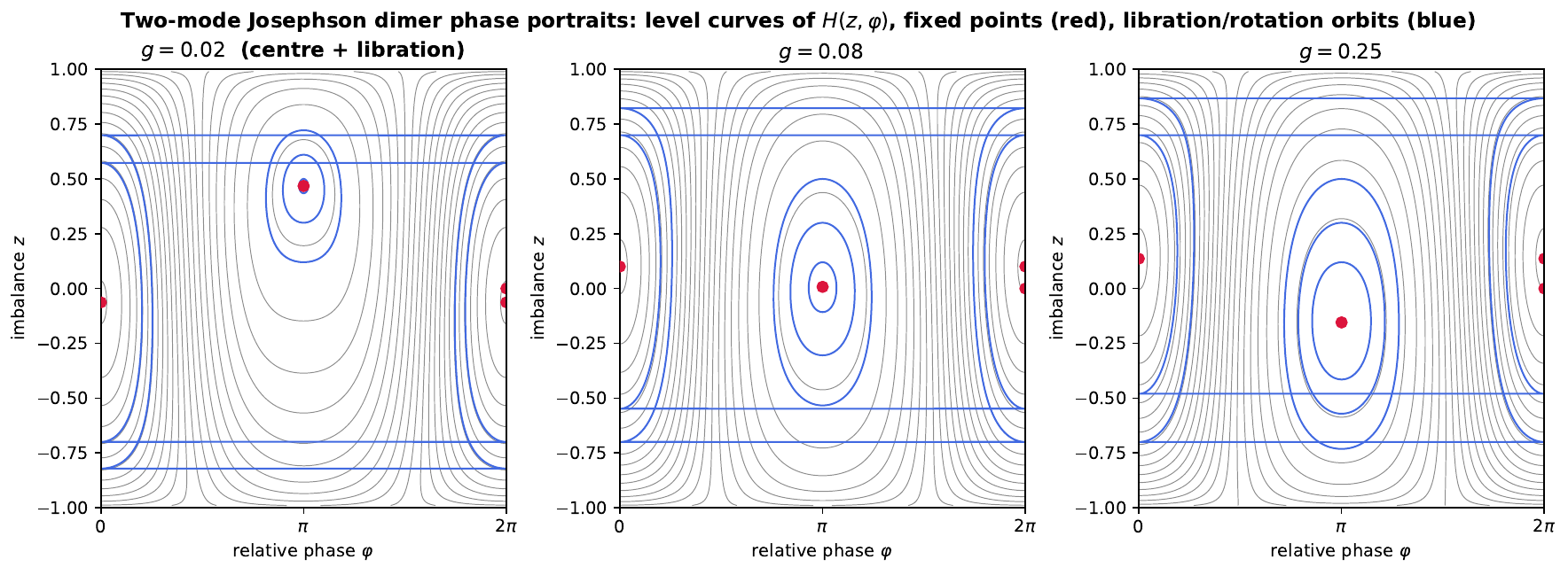
The two-mode Josephson dimer (integrable, but structurally wrong)
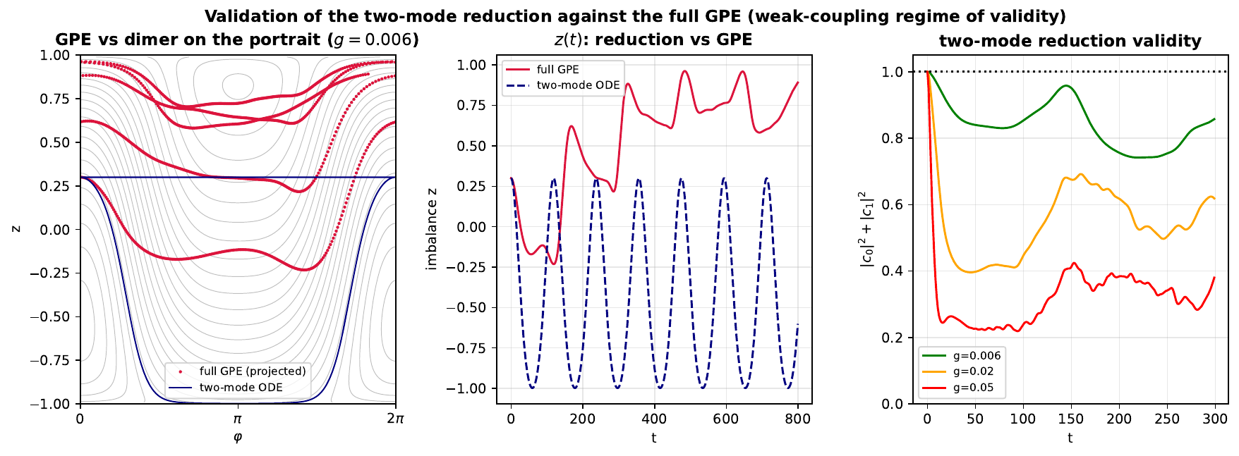
Projecting onto \(\{\phi_0,\phi_1\}\) and writing \(z=|c_0|^2-|c_1|^2\) and the relative phase \(\varphi\), the reduced one-degree-of-freedom Hamiltonian is, with overlaps \(T_{0000}=5.093\), \(T_{1111}=3.184\), \(T_{0011}=2.547\), \(T_{0001}=3.054\), \(T_{0111}=2.583\) and \(\mu_0=0.04\), \(\mu_1=0.08\), \begin{equation}H(z,\varphi)=\mu_0P_0+\mu_1P_1 +\tfrac{g}{2}\big[P_0^2T_{0000}+P_1^2T_{1111}+(s^2+2P_0P_1)T_{0011} +2(P_0T_{0001}+P_1T_{0111})s\big],\end{equation} with \(P_{0,1}=(1\pm z)/2\) and \(s=\sqrt{1-z^2}\cos\varphi\). This is an integrable bosonic Josephson dimer; its level curves are the orbits (Fig. 5, left), with an elliptic center at \(\varphi=\pi\) whose libration island inflates and migrates as \(g\) increases.
Structural failure. Crucially, because the LG modes are exact eigenstates there is no linear (Josephson) tunneling term: all coupling is nonlinear, through the asymmetric overlaps \(T_{0001},T_{0111}\). The dimer therefore omits the mode that the dynamics actually excite (Sec. 7.2), and is quantitatively valid only at weak coupling. Figure 5 (right) validates it against the full GP solver: the projected \((z,\varphi)\) trajectory agrees with the dimer ODE in the initial transfer direction but diverges once occupation leaks out of the two-mode subspace. The retained two-mode norm is \({\sim}0.7\)–\(1.0\) at \(g=0.006\) but only \({\sim}0.25\) at \(g=0.05\): the dimer is a weak-coupling caricature, not a quantitatively predictive model.
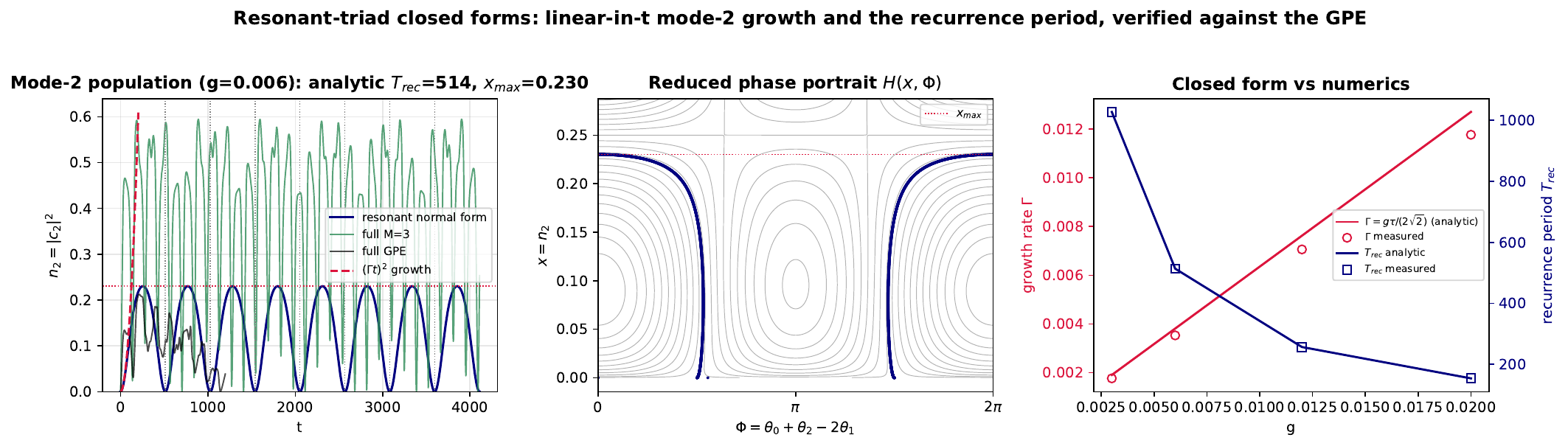
The exact internal resonance and the resonant triad
The decisive structural fact is that the spectrum \(\eqref{eq:spectrum}\) is exactly equally spaced. Hence for every \(n\) \begin{equation}\mu_n+\mu_{n+2}=2\mu_{n+1}\qquad(\text{exact, zero detuning}), \label{eq:resonance}\end{equation} and the four-wave process \(c_{n+1}c_{n+1}\leftrightarrow c_n c_{n+2}\) is secular: a pure two-mode state seeds its neighbour at any coupling, with no small-divisor protection. (Numerically \(\mu_0+\mu_2-2\mu_1=0\) to machine precision, with resonant coupling \(\tau\equiv T_{0112}=1.796\neq0\).) This is exactly the partner the dimer omits, and the structural reason it fails. The minimal faithful model is the resonant triad \(\{\phi_0,\phi_1,\phi_2\}\).
Keeping only the secular terms, the triad has two Manley–Rowe invariants—the total norm \(N=n_0+n_1+n_2\) and \(n_0-n_2\) (each four-wave event changes \((n_0,n_1,n_2)\) by \((+1,-2,+1)\)). With the equal two-mode start these reduce the problem to a single coordinate \(x\equiv n_2\): \begin{equation}n_0=\tfrac12+x,\qquad n_1=\tfrac12-2x,\qquad n_2=x\in[0,\tfrac14]. \label{eq:manleyrowe}\end{equation} In the population/phase variables \((x,\Phi)\) with \(\Phi=\theta_0+\theta_2-2\theta_1\) the reduced Hamiltonian is \begin{equation}H(x,\Phi)=D(x)+2g\tau\sqrt{n_0 n_2}\,n_1\cos\Phi,\qquad D(x)=\tfrac{g}{2}\!\sum_n T_{nnnn}n_n^2+2g\!\!\sum_{n<m}\!T_{nnmm}n_n n_m, \label{eq:Hxphi}\end{equation} with \(T_{0000},T_{1111},T_{2222}=5.093,3.184,2.397\) and \(T_{0011},T_{0022},T_{1122}=2.547,1.914,1.914\).
(i) Mode-growth rate.
Near \(x=0\) the additive drive \(i\dot c_2=g\tau\,c_0^*c_1^2\) gives linear-in-time amplitude growth, \(\sqrt{n_2}\simeq\Gamma t\), with \begin{equation}\boxed{\;\Gamma=\frac{g\tau}{2\sqrt2}\;} \label{eq:growth}\end{equation} (using \(|c_0^*c_1^2|=|c_0|\,|c_1|^2=1/(2\sqrt2)\) at the equal-weight start).
(ii) Recurrence period.
Since \(H\) is conserved and the coupling vanishes at \(x=0\) (so \(H_0=D(0)\)), the single quadrature follows, \begin{equation}\dot x=\pm\sqrt{(2g\tau)^2\,n_1^2\,n_0\,x-\big(D(x)-D(0)\big)^2},\end{equation} and the full mode-2 cycle \(x:0\to x_{\max}\to 0\) has period \begin{equation}\boxed{\;T_{\rm rec}=2\!\int_0^{x_{\max}}\!\frac{dx} {\sqrt{(2g\tau)^2\,n_1^2\,n_0\,x-\big(D(x)-D(0)\big)^2}}\;} \ \propto\ \frac1g, \label{eq:Trec}\end{equation} \(x_{\max}\) the smallest positive root of the radicand. The reduced orbit is a separatrix loop from \(x=0\) up to \(x_{\max}\) and back, which is why the mode-2 population returns as a sharp pulse train rather than a smooth oscillation; the bound \(n_2\le\tfrac14\) is the Manley–Rowe ceiling \(\eqref{eq:manleyrowe}\).
Verification.
Table 3 and Fig. 6 compare the closed forms \(\eqref{eq:growth}\)–\(\eqref{eq:Trec}\) against direct integration of the resonant normal form and of the full GP solver. The period and turning point match to four significant figures across \(g=0.003\)–\(0.02\), and \(T_{\rm rec}\propto1/g\) is confirmed; the growth rate \(\Gamma\) agrees to \({\sim}7\%\) (the residual from the slightly concave rise that the linear fit averages over).
Supplementary Animation A5.
The time parametrization of the separatrix loop—the one thing the
static Fig. 6 cannot show—is available as a 20-second
animation (online;
generated by make_anim_A5.py, which re-runs the resonant
normal form of Eq. \(\eqref{eq:Hxphi}\) at \(g=0.006\) over two recurrence periods).
Left panel: \(n_2(t)\) builds up as a
sharp pulse train, with the analytic \(T_{\rm
rec}=513.7\) gridlines and the turning point \(x_{\max}=0.2301\) marked; the trajectory
peaks exactly at the analytic ceiling. Right panel: the reduced portrait
\(H(x,\Phi)\) with the trajectory point
crawling the separatrix loop in sync—lingering near the slow
pivot at \(x\approx0\) for most of each
period, then snapping up to \(x_{\max}\) and back. Watching the
linger-and-snap makes visible why the recurrence is a pulse train rather
than a smooth oscillation: the orbit spends nearly all its time at the
pivot where the four-wave drive \(\propto\sqrt{n_2}\) is weakest.
Supplementary Animation A5 (20 s): the resonant triad lingers at the x≈0 pivot, snaps up the separatrix loop to xmax=0.230, and returns — the pulse-train recurrence with the analytic Trec=513.7 marked. Generated by make_anim_A5.py.
| \(g\) | \(\Gamma_{\rm an}\) | \(\Gamma_{\rm num}\) | \(x_{\max,\rm an}\) | \(x_{\max,\rm num}\) | \(T_{\rm rec,an}\) | \(T_{\rm rec,num}\) | |
|---|---|---|---|---|---|---|---|
| 0.003 | 0.00191 | 0.00177 | 0.2301 | 0.2301 | 1027.4 | 1027.5 | |
| 0.006 | 0.00381 | 0.00353 | 0.2301 | 0.2301 | 513.7 | 513.7 | |
| 0.012 | 0.00762 | 0.00706 | 0.2301 | 0.2301 | 256.8 | 256.8 | |
| 0.020 | 0.01270 | 0.01176 | 0.2301 | 0.2301 | 154.1 | 154.1 |
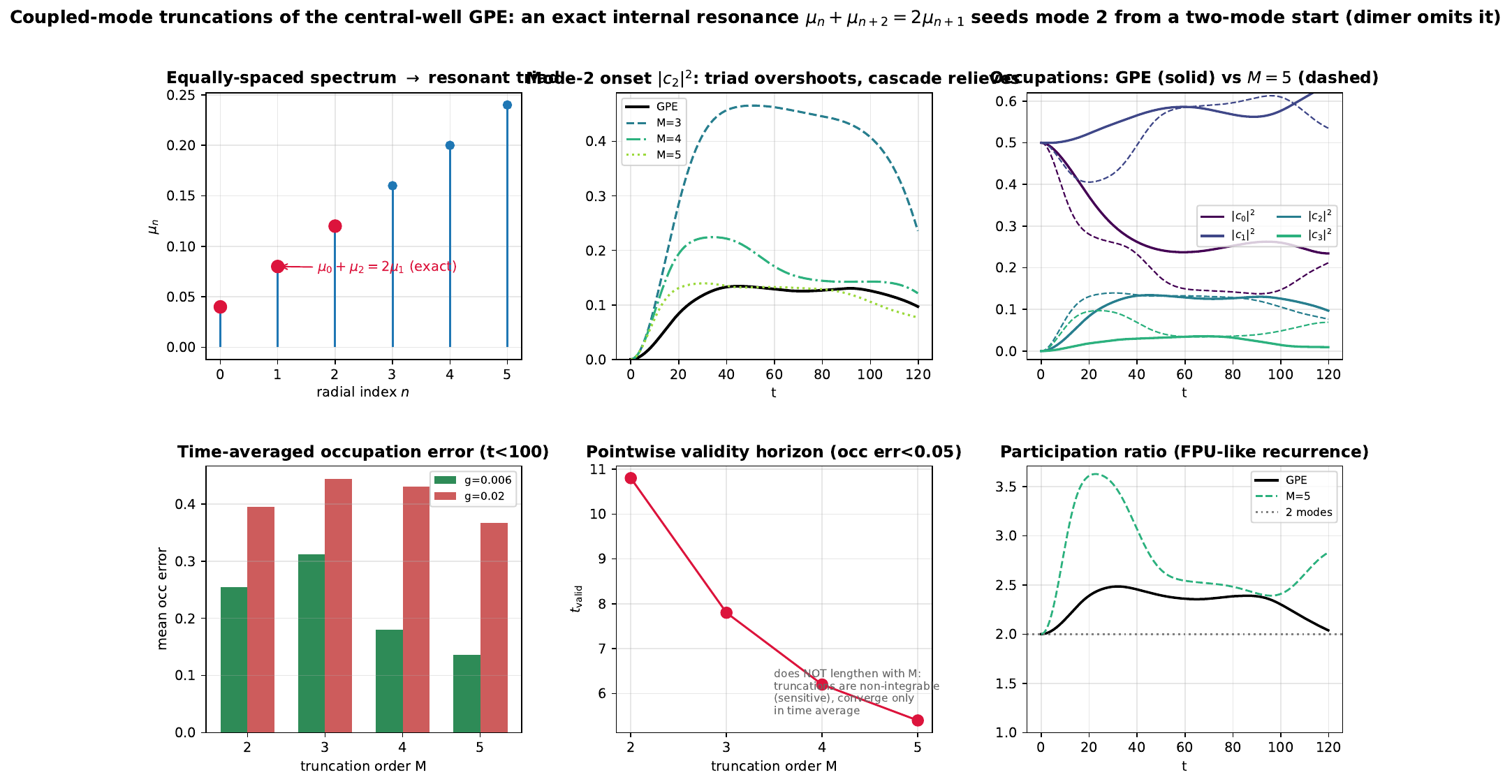
From triad to cascade: convergence of truncations
Because the resonance \(\eqref{eq:resonance}\) repeats up the entire ladder, energy does not stop at mode 2. Figure 7 examines \(M\)-mode coupled-mode truncations of the full solver. The minimal triad (\(M=3\)) captures the mode-2 onset but overshoots its amplitude, because a closed triad has nowhere downstream to shed flux; adding modes (\(M=4,5\)) relieves the overshoot via the cascade. The truncations converge in time-averaged occupation (mean error \(0.26\to0.14\) from \(M=2\) to \(5\) at \(g=0.006\)), but the pointwise validity horizon does not lengthen with \(M\) (it shortens, \(t_{\rm valid}:10.8\to5.4\)): successive truncations sit on slightly different invariant tori (their amplitudes dephase linearly; this is not chaotic divergence, cf. Sec. 7.4), so they agree statistically rather than trajectory-by-trajectory. This is the dimer\(\to\)triad\(\to\)cascade hierarchy.
Nonlinear normal modes and the near-integrability of the dynamics
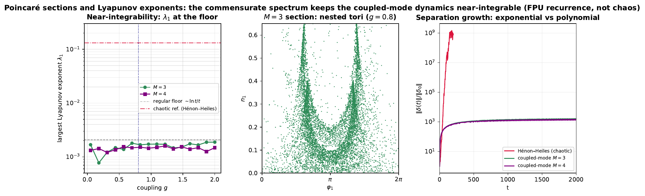
The fixed-point states are the elliptic centers that the periodic orbits encircle; they are the Lyapunov continuation of the linear eigenstates to finite \(g\) (nonlinear normal modes). It is natural to ask whether, with three or more strongly coupled modes, the system becomes chaotic. We tested this directly with the largest Lyapunov exponent \(\lambda_1\) (two-trajectory Benettin method [16], RK4 projected onto \(|c|=1\)) and with Poincaré sections of the reduced flow (Fig. 8). The estimator is validated on the Hénon–Heiles Hamiltonian, where it returns \(\lambda_1\approx0.13\) at a chaotic energy and the linear-separation floor \(\approx 0.001\) at a regular one.
The result is that the coupled-mode dynamics remain near-integrable. For both \(M=3\) and \(M=4\), \(\lambda_1\) stays at the regular floor (\(\sim\!\ln t/t\), i.e. \(\lesssim2\times10^{-3}\)) across the entire range \(g\in[0.05,2]\)—more than sixty times below the chaotic reference—and the tangent separation grows only polynomially (\(\delta(t)/\delta_0\sim10^3\) at \(t=2000\)) rather than exponentially (Fig. 8, right, where the Hénon–Heiles reference reaches \(10^9\)). The \(M=3\) Poincaré section is a family of nested invariant tori. The origin of this robustness is the exact commensurability of the spectrum: rather than a few isolated resonances that broaden and overlap (the Chirikov route to chaos), the equally spaced ladder makes all four-wave terms resonant at zero detuning, a highly non-generic, near-integrable structure. This is precisely why the FPU recurrence of Secs. 4–5 is so robust: the system does not thermalize because it is dynamically close to an integrable one, the same mechanism that underlies the original Fermi–Pasta–Ulam–Tsingou observation. Correspondingly, the non-monotone truncation behaviour of Fig. 7 reflects that successive truncations sit on slightly different tori—so their trajectories dephase linearly—rather than any exponential (chaotic) divergence.
Supplementary Animation A6.
The contrast is available as a 15-second animation (online;
generated by make_anim_A6.py, which re-runs the Fig. 8 computations unmodified). Left: the
tangent-separation race on a log axis—the Hénon–Heiles reference rockets
exponentially to \({\sim}10^9\) within
the opening moments of the movie, while the \(M=3\) and \(M=4\) coupled-mode curves crawl
polynomially for the remaining duration and saturate near \(10^3\), six orders of magnitude below.
Right: the \(M=3\) Poincaré section
accumulates crossing by crossing, each trajectory tracing out its own
closed invariant curve—regularity assembling itself point by point. The
pacing itself carries the physics: exponential versus polynomial growth
is precisely a statement about how fast things happen.
Supplementary Animation A6 (15 s): the tangent-separation race — Hénon–Heiles rockets exponentially to 109 while the coupled-mode systems crawl polynomially to 103; the M=3 Poincaré section accumulates into nested invariant tori. Generated by make_anim_A6.py.
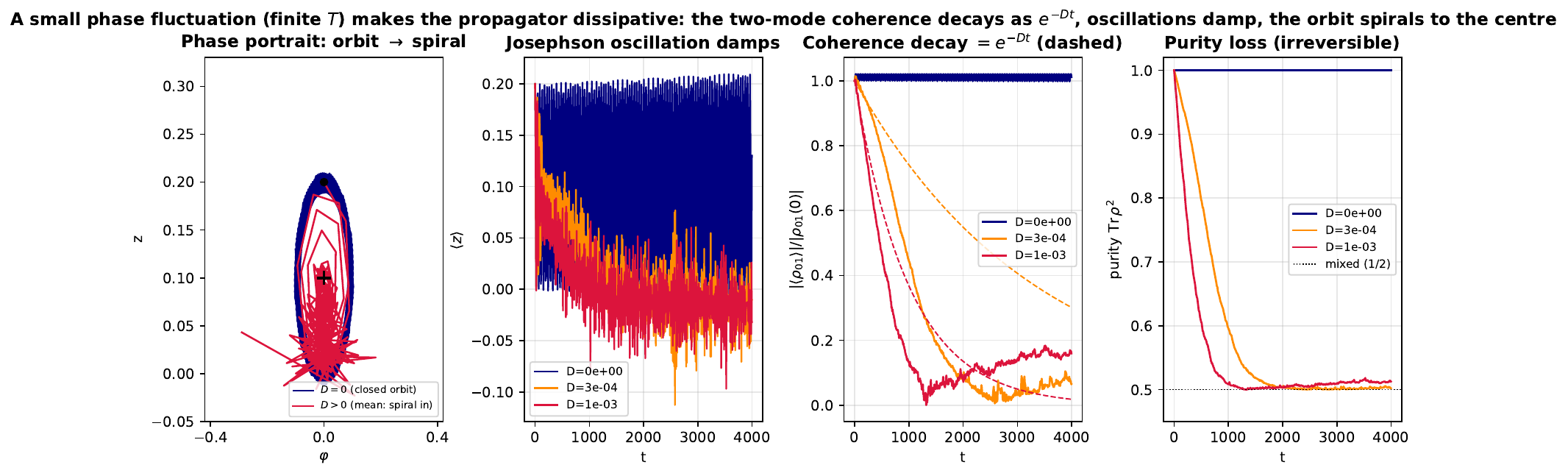
Finite-temperature dissipation and the fixed point as attractor
The dynamics above are conservative, so they have no attractors—only periodic orbits and the near-integrable recurrence. The imaginary-time companion study, by contrast, has the LG modes as genuine attractors. The bridge between the two is dissipation, and the physical source of dissipation in this framework is temperature understood as phase de-locking: a finite temperature is a small stochastic fluctuation of the phase field. We show here that such a fluctuation makes the propagator dissipative, that it turns the conservative orbits into attractors, and that—once the fluctuation is paired with its fluctuation–dissipation partner—the dynamics relax to a thermal cloud about the imaginary-time fixed point, recovering that fixed point exactly as the \(T\to0\) attractor.
A phase fluctuation is a dissipative multiplier
Let each step multiply the field by a small random local phase, \(\psi(\mathbf r)\to\psi(\mathbf r)\,e^{i\xi(\mathbf r)}\) with \(\langle\xi\rangle=0\) and \(\langle\xi^2\rangle=\sigma^2\propto T\). The pointwise density \(|\psi|^2\) is unchanged, so the norm is conserved in every realization; but the coherent (ensemble-averaged) field acquires a real multiplier, because for Gaussian \(\xi\) \begin{equation}\langle e^{i\xi}\rangle = e^{-\sigma^2/2}\equiv e^{-D\,\delta t}, \qquad D=\frac{\sigma^2}{2\,\delta t}\propto T . \label{eq:multiplier}\end{equation} The unitary propagator thus picks up a non-unitary factor \(e^{-D\delta t}<1\) that damps coherences, not populations: \(D\) is a decoherence rate set by temperature. In the two-mode reduction this is phase diffusion of the relative phase, \begin{equation}\dot z=-2\,\partial_\varphi H,\qquad d\varphi = 2\,\partial_z H\,dt + \sqrt{2D}\,dW, \label{eq:stochdimer}\end{equation} and Itô’s lemma gives \(d\langle e^{i\varphi}\rangle/dt=(\text{drift}) -D\langle e^{i\varphi}\rangle\): the off-diagonal coherence \(\rho_{01}\propto\langle e^{i\varphi}\rangle\) decays at rate \(D\).
An ensemble integration of Eq. \(\eqref{eq:stochdimer}\) (Fig. 9) confirms the consequences. The coherence \(|\langle\rho_{01}\rangle|\) decays exactly as the dissipative multiplier \(e^{-Dt}\); the Josephson population oscillation of \(\langle z\rangle\) damps to zero; the purity \(\operatorname{Tr}\rho^2\) falls from \(1\) to the maximally mixed value \(1/2\) irreversibly (no recurrence, in sharp contrast with the conservative case of Secs. 4–5); and in the \((\varphi,z)\) portrait the conservative closed orbit becomes an inward spiral—the elliptic center becomes a weak attractor. Pure phase noise, however, only dephases: it damps coherence and oscillation but, lacking an energy-relaxation channel, drives the state to the maximally mixed diagonal ensemble at the current energy rather than to a definite state.
Supplementary Animation A7.
The decoherence mechanism is available as a 15-second animation (online;
generated by make_anim_A7.py, which re-runs the Eq. \(\eqref{eq:stochdimer}\) ensemble unmodified).
Two \((\varphi,z)\) portraits play side
by side, each carrying an ensemble of \(250\) trajectories started from a small
blob on a libration orbit. At \(D=0\)
the cloud shears into a dotted ring along the closed orbit (classical
phase mixing) but never leaves it, and the coherence stays at unity for
the entire run—Hamiltonian flow does not decohere. At \(D=3\times10^{-4}\) the same cloud diffuses,
the coherence collapses (the multiplier \(e^{-Dt}\) is the envelope; the blob start
adds shear-enhanced decay on top of it, down to the finite-ensemble
floor \({\sim}1/\sqrt{N_{\rm
traj}}\)), and the ensemble mean (crimson trail) spirals
into the elliptic center: the moment the orbit becomes an attractor,
watched directly. The contrast between the panels isolates what the time
traces of Fig. 9 alone cannot—that the decay is
entirely the noise’s doing, not the flow’s.
Supplementary Animation A7 (15 s): a 250-trajectory ensemble on the dimer portrait. At D=0 the cloud shears along the closed orbit (reversible phase mixing); at D>0 it diffuses, the coherence decays as e−Dt, and the ensemble mean spirals into the center. Generated by make_anim_A7.py.
The fluctuation–dissipation balance and the \(T\to0\) attractor
To reach a definite thermal state, the fluctuation must be paired with its dissipative partner via the fluctuation–dissipation theorem (FDT). This is the stochastic projected Gross–Pitaevskii equation (SPGPE) [26, 27, 28], which in the mode basis reads \begin{equation}dc_n = \underbrace{-i F_n\,dt}_{\text{Hamiltonian}} \;\underbrace{-\,\gamma\,(F_n-\mu_{\rm eff}c_n)\,dt}_{\text{damping}=\text{ imaginary time}} \;+\;\underbrace{dW_n}_{\text{noise}},\qquad \langle dW_n\,dW_m^*\rangle = 2\gamma T\,\delta_{nm}\,dt, \label{eq:spgpe}\end{equation} with the force \(F_n=\mu_n c_n+g\sum_{jkl}T_{njkl}c_j^*c_kc_l\), instantaneous chemical potential \(\mu_{\rm eff}=\mathrm{Re}\,\langle c|F\rangle/\langle c|c\rangle\), and the norm fixed to unity each step (number-conserving projected GPE; the truncated LG basis is the projector that regularizes the Rayleigh–Jeans ultraviolet catastrophe). The damping term is precisely the normalized imaginary-time gradient flow on the energy, and the noise strength \(2\gamma T\) is locked to the damping \(\gamma\) by FDT, so the stationary measure is the classical-field Gibbs ensemble \(P[\psi]\propto e^{-(E[\psi]-\mu N)/T}\).
At \(T=0\) the noise vanishes and Eq. \(\eqref{eq:spgpe}\) is exactly imaginary-time relaxation. Figure 10 shows that it converges, from many random initial conditions, to the same fixed point—the nonlinear ground state \(\phi_{0,1}\) (condensate occupation \(0.97\)), with \(E(t)-E_{\min}\to10^{-13}\): the universal \(T\to0\) attractor. At \(T>0\) the system equilibrates to a thermal cloud about that fixed point, and two quantitative checks confirm it is the correct Gibbs state rather than generic spreading. First, classical-field equipartition: each quadratic fluctuation mode carries energy \(T\), so \(E_{\rm ss}-E_{\min}=(\text{\# excited modes})\times T\) and \((\langle|c_n|^2\rangle-n_n^{\rm fix})(\mu_n-\mu_0)=T\) across modes (Rayleigh–Jeans). Second, the thermal depletion of the condensate is linear in \(T\) with slope \(\sum_{n>0}(\mu_n-\mu_0)^{-1}\) and extrapolates to zero as \(T\to0\): the cloud shrinks continuously onto the fixed point. The fixed point of the dissipative flow is thus recovered exactly as the zero-temperature limit of the finite-temperature dynamics.
Supplementary Animation A8.
The two limits of Fig. 10 are available as a 24-second, two-act
animation (online;
generated by make_anim_A8.py, which reuses the Eq. \(\eqref{eq:spgpe}\) integrator unmodified and adds
only the real-space reconstruction \(\psi=\sum_n c_n\phi_n\) per frame). Act
1 (\(T=0\)): five random initial
fields \(|\psi|^2\) evolve under the
FDT damping—which at zero noise is exactly imaginary-time flow—while
\(E(t)-E_{\min}\) descends on a log
axis; the five visibly different starting profiles morph into the
same fixed-point ring, the dynamical meaning of a universal
attractor. Act 2 (temperature ladder): the steady-state field
is shown at \(T=0.003\to0.0015\to0.0006\to0\), side by
side with the depletion-vs-\(T\) line
of Fig. 10; the thermal speckle visibly freezes
out as a marker walks down the equipartition line and lands on the fixed
point at \(T=0\). Parameters as in
Fig. 10 (\(g=0.003\), \(\gamma=0.5\), \(\Delta t=0.05\), six modes; run parameters
embedded in the video metadata).
Supplementary Animation A8 (24 s, two acts): five random fields converge to the same fixed point at T=0; the thermal cloud freezes out onto it as T→0. Generated by make_anim_A8.py.
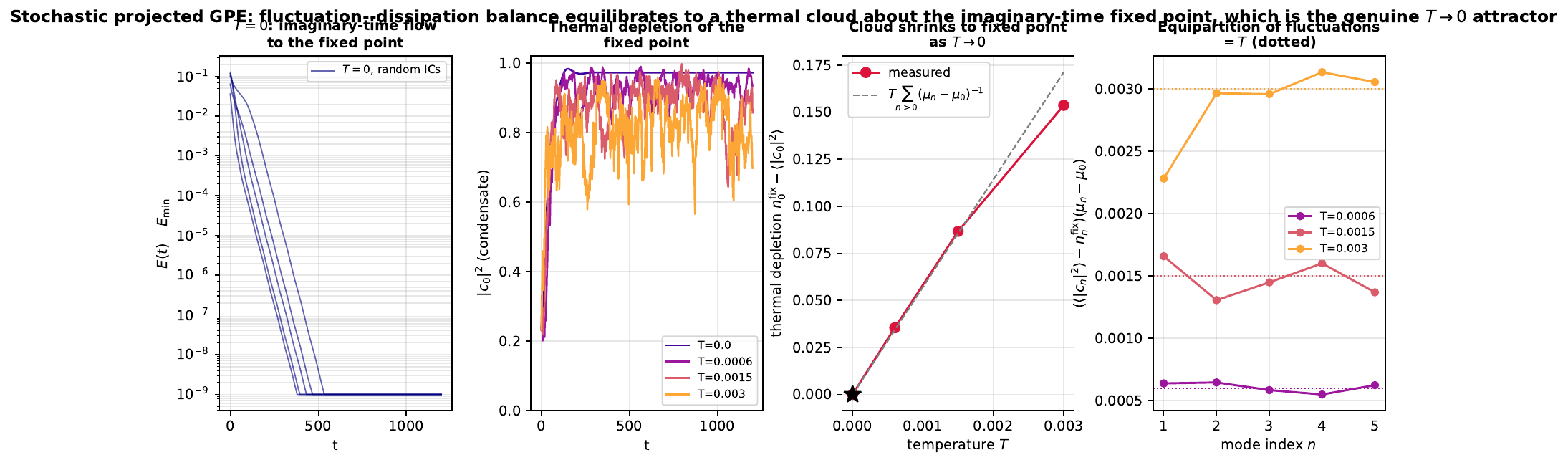
The conservative–dissipative family.
Temperature interpolates a single family, with \(D\propto T\) the control knob. At \(T=0\) with no damping the dynamics are conservative: periodic orbits, no attractor, recurrent coherence (Secs. 3–7). Pure phase noise adds decoherence (coherence \(\to0\) as \(e^{-Dt}\)) but no energy relaxation, giving the maximally mixed ensemble (Sec. 8.1). The FDT-complete dissipation relaxes the system to the Gibbs cloud about the imaginary-time fixed point (Sec. 8.2), and the \(T\to0\) limit recovers that fixed point exactly. The shell-selecting attractors of the imaginary-time study are therefore the zero-temperature attractors of the physical, finite-temperature dynamics—not artifacts of the gradient flow.
Discussion
Two faces of the fixed point.
The same LG mode is a dissipative attractor under imaginary time and the elliptic center of conservative periodic orbits under real time. The real-time orbits are, loosely, the imaginary-time relaxation “run as Hamiltonian flow”; adding dissipation collapses the periodic orbits onto the fixed points (Sec. 8), recovering the shell-selecting mechanism of the companion study. “Limit cycle” in the conservative setting must therefore be read as “periodic orbit”; a genuine attracting cycle requires dissipation, and Sec. 8 supplies it physically as finite temperature (phase de-locking), recovering the fixed point as the \(T\to0\) attractor.
Physical vs numerical.
Every claim here rests on the verified, norm- and energy-conserving propagator. We deliberately avoid the de-aliasing mask (which would break unitarity) and any renormalization (which would inject or remove norm); the conservation budgets in Table 1 and the four-figure agreement in Table 3 are the evidence that the redistribution and recurrence are physical, not artifacts of the discretization.
Limitations.
The treatment is two-dimensional, single central potential, fixed-\(m\) sector, and mean-field (no quantum depletion). The high-end participation ratio is truncation-limited by the finite mode basis. The resonant-triad closed forms assume the secular (rotating-wave) reduction; the full solver carries an additional fast non-resonant ripple that breaks the Manley–Rowe invariants and lets bare low-\(M\) truncations overshoot the \(n_2\le\tfrac14\) ceiling.
Conclusion
Real-time superpositions of central-well LG modes redistribute but do not relax. The linear motion is exactly periodic (commensurate spectrum, full revival at \(\pi/(2\sqrt\kappa)\)) and the nonlinearity generates modes within a bounded, recurrent budget—FPU recurrence rather than relaxation—while the modal density matrix dephases into a mixed diagonal ensemble whose inverse purity is the participation ratio. The analytically tractable hierarchy is now complete: the two-mode dimer is integrable but structurally blind to the dynamics, because the exactly equally-spaced spectrum makes \(\mu_n+\mu_{n+2}=2\mu_{n+1}\) a secular resonance; the resonant triad is the minimal faithful model, with closed-form mode-growth rate \(\Gamma=g\tau/(2\sqrt2)\) and recurrence period \(T_{\rm rec}\propto1/g\) verified to four significant figures; and the resonance repeats up the ladder to give a cascade whose truncations converge only in time average. Lyapunov exponents and Poincaré sections show the dynamics remain near-integrable rather than chaotic—the commensurate spectrum makes every four-wave term resonant, a non-generic structure that suppresses thermalization and so underlies the robust recurrence. Genuine limit cycles, and the shell-selecting attractors, require dissipation: a small phase fluctuation (finite temperature) supplies it, and with its fluctuation–dissipation partner the dynamics relax to a thermal cloud about the imaginary-time fixed point, recovering it exactly as the \(T\to0\) attractor and closing the conservative–dissipative loop.
The coupling tensor
For a fixed-\(m\) sector the four-mode overlap reduces to the real, fully symmetric tensor \(T_{pqrs}=\int R_pR_qR_rR_s\,d^2x\) of Eq. \(\eqref{eq:Ttensor}\). Its diagonal (\(T_{nnnn}\), self-phase modulation) and pair (\(T_{nnmm}\), cross-phase modulation) entries fix the diagonal energy \(D(x)\) of Eq. \(\eqref{eq:Hxphi}\); the off-diagonal entry \(\tau=T_{0112}\) is the resonant four-wave coupling. Selection rules follow from the angular integral (all combinations allowed within a fixed-\(m\) sector) and from the radial overlaps decaying with mode-index separation. Numerically (for the parameters of Sec. 2) \(T_{0000}=5.093\), \(T_{1111}=3.184\), \(T_{2222}=2.397\), \(T_{0011}=2.547\), \(T_{0022}=1.914\), \(T_{1122}=1.914\), \(\tau=T_{0112}=1.796\).
The resonant-triad normal form
Writing \(c_n=\sqrt{n_n}\,e^{i\theta_n}\) and inserting the secular reduction \(\eqref{eq:manleyrowe}\) into the coupled-mode equations gives the single canonical pair \((x,\Phi)\) with Hamiltonian \(\eqref{eq:Hxphi}\). The equation of motion \(\dot x=-\partial H/\partial\Phi=2g\tau\,n_1\sqrt{n_0 n_2}\,\sin\Phi\) combined with energy conservation \(H(x,\Phi)=D(0)\) eliminates \(\Phi\) and yields the quadrature \(\eqref{eq:Trec}\). The turning point \(x_{\max}\) is the smallest positive root of the radicand; for the present parameters \(x_{\max}=0.230\), just below the Manley–Rowe ceiling \(\tfrac14\), so the orbit is a separatrix loop and the recurrence is a sharp pulse train. The small-\(x\) expansion of the additive drive gives the growth rate \(\eqref{eq:growth}\).
Numerical methods and conservation
All real-space dynamics use the Strang split-step Fourier
propagator [32, 33]: a half-step of the diagonal
(potential\(+\)nonlinear) operator
\(\exp[-i(V+gN^2|\psi|^2)\,\Delta
t/2]\), a full spectral kinetic step \(\exp(-i|\mathbf k|^2\Delta t)\), and a
second diagonal half-step. The scheme is exactly unitary (no de-aliasing
mask, no renormalization), giving norm drift \(\lesssim10^{-12}\) and energy drift \(\lesssim10^{-7}\) over the runs reported.
Modal occupations are obtained by projection onto the grid-normalized LG
modes \(\eqref{eq:lg}\). Reduced (coupled-mode and
resonant-normal-form) systems are integrated with an adaptive high-order
Runge–Kutta (DOP853, tolerances \(10^{-11}/10^{-13}\)), conserving the norm
to \(\lesssim10^{-8}\). Parameters:
\(m=1\), \(\kappa=10^{-4}\), \(N=160\), \(L=80\), \(\Delta
t\in[0.01,0.05]\). Reproduction scripts:
analyze_superposition_dynamics.py (Sec. 4),
make_linear_density.py (Secs. 3,5), make_dimer_portrait.py
(dimer), make_three_mode.py (cascade),
triad_analytics.py (closed forms),
make_chaos.py (Lyapunov/Poincaré, Sec. 7.4),
make_fate_gallery.py (gallery, Sec. 6; its
eigenstates from imaginary-time relaxation with Gram–Schmidt),
make_phase_noise.py (stochastic dimer, Sec. 8.1), and make_spgpe.py
(SPGPE, Sec. 8.2). Supplementary Animations A1–A5, A7,
and A8 are generated by make_anim_A1.py through
make_anim_A8.py, which re-run the corresponding evolution
loops unmodified and only add frame capture (and, for A1 and A8, the
real-space reconstruction \(\sum_n
c_n\phi_n\)). Lyapunov exponents use the two-trajectory Benettin
method with RK4 projected onto \(|c|=1\) and periodic renormalization,
validated against the Hénon–Heiles system; Poincaré sections record
\(\varphi_2=0\) up-crossings on
fixed-energy initial data. The stochastic models are integrated by
Euler–Maruyama (symplectic semi-implicit for the dimer Hamiltonian part)
over ensembles of \(\sim\!600\)
realizations; the SPGPE uses \(\gamma=0.5\), fixed norm, and
time/realization averaging over the second half of each run for
steady-state statistics.
References
[1] F. Dalfovo, S. Giorgini, L. P. Pitaevskii, S. Stringari, Theory of Bose–Einstein condensation in trapped gases, Rev. Mod. Phys.\ 71, 463 (1999). doi:10.1103/RevModPhys.71.463
[2] C. J. Pethick, H. Smith, Bose–Einstein Condensation in Dilute Gases, 2nd ed., Cambridge University Press (2008). doi:10.1017/CBO9780511802850
[3] L. P. Pitaevskii, S. Stringari, Bose–Einstein Condensation and Superfluidity, Oxford University Press (2016). doi:10.1093/acprof:oso/9780198758884.001.0001
[4] L. Allen, M. W. Beijersbergen, R. J. C. Spreeuw, J. P. Woerdman, Orbital angular momentum of light and the transformation of Laguerre–Gaussian laser modes, Phys. Rev. A 45, 8185 (1992). doi:10.1103/PhysRevA.45.8185
[5] A. L. Fetter, Rotating trapped Bose–Einstein condensates, Rev. Mod. Phys. 81, 647 (2009). doi:10.1103/RevModPhys.81.647
[6] A. Smerzi, S. Fantoni, S. Giovanazzi, S. R. Shenoy, Quantum coherent atomic tunneling between two trapped Bose–Einstein condensates, Phys. Rev. Lett. 79, 4950 (1997). doi:10.1103/PhysRevLett.79.4950
[7] S. Raghavan, A. Smerzi, S. Fantoni, S. R. Shenoy, Coherent oscillations between two weakly coupled Bose–Einstein condensates: Josephson effects, π oscillations, and macroscopic quantum self-trapping, Phys. Rev. A 59, 620 (1999). doi:10.1103/PhysRevA.59.620
[8] G. J. Milburn, J. Corney, E. M. Wright, D. F. Walls, Quantum dynamics of an atomic Bose–Einstein condensate in a double-well potential, Phys. Rev. A 55, 4318 (1997). doi:10.1103/PhysRevA.55.4318
[9] M. Albiez et al., Direct observation of tunneling and nonlinear self-trapping in a single bosonic Josephson junction, Phys. Rev.\ Lett. 95, 010402 (2005). doi:10.1103/PhysRevLett.95.010402
[10] R. Gati, M. K. Oberthaler, A bosonic Josephson junction, J. Phys. B 40, R61 (2007). doi:10.1088/0953-4075/40/10/R01
[11] J. C. Eilbeck, M. Johansson, The discrete nonlinear Schrödinger equation—20 years on, in Localization and Energy Transfer in Nonlinear Systems, World Scientific (2003), p. 44. doi:10.1142/9789812704627_0003
[12] P. G. Kevrekidis, The Discrete Nonlinear Schrödinger Equation, Springer (2009). doi:10.1007/978-3-540-89199-4
[13] E. Fermi, J. Pasta, S. Ulam, Studies of nonlinear problems, Los Alamos Report LA-1940 (1955); reprinted in Collected Papers of Enrico Fermi, Vol. II. doi:10.2172/4376203
[14] G. P. Berman, F. M. Izrailev, The Fermi–Pasta–Ulam problem: fifty years of progress, Chaos 15, 015104 (2005). doi:10.1063/1.1855036
[15] G. Gallavotti (ed.), The Fermi–Pasta–Ulam Problem: A Status Report, Lect. Notes Phys. 728, Springer (2008). doi:10.1007/978-3-540-72995-2
[16] G. Benettin, L. Galgani, A. Giorgilli, J.-M. Strelcyn, Lyapunov characteristic exponents for smooth dynamical systems and for Hamiltonian systems; a method for computing all of them, Meccanica 15, 9 (1980). doi:10.1007/BF02128236
[17] B. V. Chirikov, A universal instability of many-dimensional oscillator systems, Phys. Rep. 52, 263 (1979). doi:10.1016/0370-1573(79)90023-1
[18] M. Hénon, C. Heiles, The applicability of the third integral of motion: some numerical experiments, Astron. J. 69, 73 (1964). doi:10.1086/109234
[19] R. W. Robinett, Quantum wave packet revivals, Phys.\ Rep. 392, 1 (2004). doi:10.1016/j.physrep.2003.11.002
[20] I. Sh. Averbukh, N. F. Perelman, Fractional revivals: universality in the long-term evolution of quantum wave packets, Phys. Lett. A 139, 449 (1989). doi:10.1016/0375-9601(89)90943-2
[21] L. Deng et al., Four-wave mixing with matter waves, Nature 398, 218 (1999). doi:10.1038/18395
[22] M. Rigol, V. Dunjko, M. Olshanii, Thermalization and its mechanism for generic isolated quantum systems, Nature 452, 854 (2008). doi:10.1038/nature06838
[23] A. Polkovnikov, K. Sengupta, A. Silva, M. Vengalattore, Colloquium: Nonequilibrium dynamics of closed interacting quantum systems, Rev. Mod. Phys. 83, 863 (2011). doi:10.1103/RevModPhys.83.863
[24] W. Kohn, Cyclotron resonance and de Haas–van Alphen oscillations of an interacting electron gas, Phys. Rev. 123, 1242 (1961). doi:10.1103/PhysRev.123.1242
[25] J. F. Dobson, Harmonic-potential theorem: implications for approximate many-body theories, Phys. Rev. Lett. 73, 2244 (1994). doi:10.1103/PhysRevLett.73.2244
[26] H. T. C. Stoof, Coherent versus incoherent dynamics during Bose–Einstein condensation in atomic gases, J. Low Temp. Phys.\ 114, 11 (1999). doi:10.1023/A:1021897703053
[27] C. W. Gardiner, M. J. Davis, The stochastic Gross–Pitaevskii equation: II, J. Phys. B 36, 4731 (2003). doi:10.1088/0953-4075/36/23/010
[28] P. B. Blakie, A. S. Bradley, M. J. Davis, R. J. Ballagh, C. W. Gardiner, Dynamics and statistical mechanics of ultra-cold Bose gases using c-field techniques, Adv. Phys. 57, 363 (2008). doi:10.1080/00018730802564254
[29] S. P. Cockburn, N. P. Proukakis, The stochastic Gross–Pitaevskii equation and some applications, Laser Phys. 19, 558 (2009). doi:10.1134/S1054660X09040057
[30] N. P. Proukakis, B. Jackson, Finite-temperature models of Bose–Einstein condensation, J. Phys. B 41, 203002 (2008). doi:10.1088/0953-4075/41/20/203002
[31] W. Bao, Q. Du, Computing the ground state solution of Bose–Einstein condensates by a normalized gradient flow, SIAM J. Sci. Comput.\ 25, 1674 (2004). doi:10.1137/S1064827503422956
[32] J. A. C. Weideman, B. M. Herbst, Split-step methods for the solution of the nonlinear Schrödinger equation, SIAM J. Numer. Anal.\ 23, 485 (1986). doi:10.1137/0723033
[33] W. Bao, S. Jin, P. A. Markowich, On time-splitting spectral approximations for the Schrödinger equation in the semiclassical regime, J.\ Comput. Phys. 175, 487 (2002). doi:10.1006/jcph.2001.6956
[34] S. A. Orszag, On the elimination of aliasing in finite-difference schemes by filtering high-wavenumber components, J. Atmos.\ Sci. 28, 1074 (1971). doi:10.1175/1520-0469(1971)028
[35] Distinguishing physical structure from grid-seeded artifacts in split-step solvers for the 2D GPE, companion study, this project.
[36] The shell-generating fixed point: an analytical treatment of the coherence quantization mechanism, companion study, this project.