CFT Deep Dive: Helium
Coherence Field Theory Deep Dive
Helium
From Two-Electron Quantum Mechanics to
Superfluid Phases and Relativistic Corrections
Paul-Jean Letourneau Starling Systems May 2026
Scope. This document is an analytical outline for a deep investigation of coherence field theory (CFT) applied to the helium atom and its condensed-matter phases. It organises the physical questions, the benchmarks against known results, and the genuinely open problems into a structured research programme. The document proceeds from atomic physics fundamentals (Part I–II), through CFT reformulation (Part III), to quantitative predictions and their comparison with established quantum chemistry (Part IV–V), relativistic and QED corrections (Part VI), isotope effects in \({}^3\mathrm{He}\) and \({}^4\mathrm{He}\) (Part VII), superfluid phases and liquid helium (Part VIII), and unsolved problems together with a research agenda (Part IX).
Philosophy. Helium is the minimal non-trivial atom: two electrons, full spherical symmetry, no permanent dipole, yet rich enough to exhibit electron correlation, exchange splitting, spin statistics, and macroscopic quantum coherence. It is therefore the ideal proving ground for any new framework claiming to supersede standard quantum mechanics. If CFT cannot reproduce the helium ground-state energy to chemical accuracy (\(< 1\,\mathrm{kcal/mol} \approx 43\,\mu \mathrm{Ha}\)), it fails at the first serious test. If it can, then the questions that follow are correspondingly ambitious.
Part I —Primer on Helium
Physics
The Helium Atom: Structure and Hamiltonian
The helium atom is the simplest many-electron system. Its non-relativistic Hamiltonian is known exactly; the challenge is that no analytical solution exists because of the interelectronic repulsion term. This irreducible two-body interaction is the engine of nearly every non-trivial effect in helium physics.
Before the machinery, it is worth seeing the object itself. The
two-electron coherence field \(\psi(\mathbf{r}_1,\mathbf{r}_2)\) lives in
six dimensions, so any single real-space picture is a projection; the
choice of projection is what makes the interelectronic repulsion visible
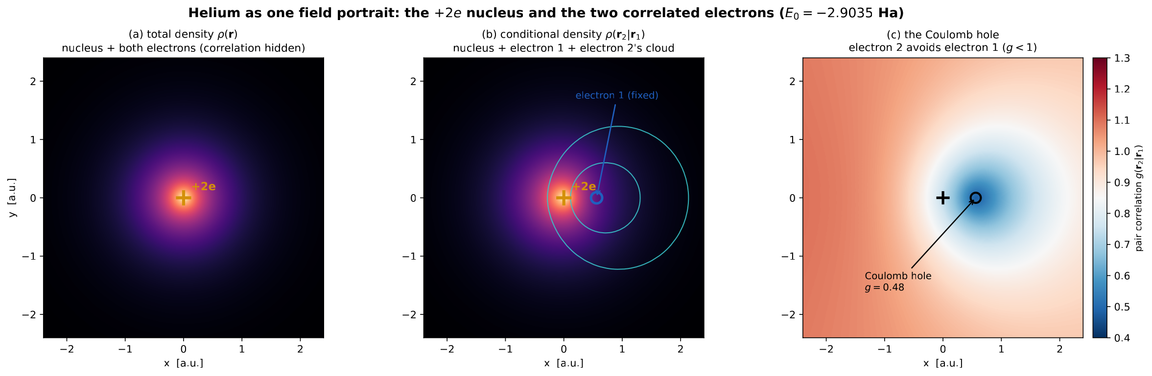
or not. Figure 1 places the nucleus and both
electrons in one frame three ways. The total density \(\rho(\mathbf{r})\) shows the \(+2e\) nucleus dressed by a single smeared
cloud—correct, but with the two electrons made indistinguishable and the
correlation integrated away. The conditional density \(\rho(\mathbf{r}_2|\mathbf{r}_1)\) pins one
electron at the shell radius and renders the other in the field of
both the nucleus and its partner, putting all three bodies in a
single real-space frame. The correlation that the total density hides
then appears explicitly as the pair-correlation factor \(g(\mathbf{r}_2|\mathbf{r}_1)\): a Coulomb
hole of depth \(g\approx0.5\) carved
into electron 2’s distribution at the position of electron 1. That
hole—the electrons’ mutual avoidance—is the real-space signature of the
repulsion term, and reproducing it is the whole content of the
two-electron problem (Sec. 7.3).
For the \({}^1\!S_0\) ground state the
Madelung phase is flat (\(\psi\) real),
so the portrait is pure amplitude, consistent with the ground state
being a pure-amplitude fixed point. The portrait is naturally dynamic:
as electron 1 is carried around the nucleus, electron 2’s Coulomb hole
tracks it—an animated version
(make_anim_He_field_portrait.py) accompanies this figure
online at coherencefield.xyz/helium/deep-dive.
analysis/helium_field_portrait.py.make_anim_He_field_portrait.py.Nuclear and electronic structure
Nucleus: charge \(Z = 2\); two stable isotopes \({}^4\mathrm{He}\) (spin-0 boson, \(99.999\,\%\) natural abundance) and \({}^3\mathrm{He}\) (spin-\(\tfrac{1}{2}\) fermion, rare).
Two electrons with mass \(m_e\), charge \(-e\), spin \(s = \tfrac{1}{2}\).
Total electronic spin \(S \in \{0, 1\}\) determines whether the atom is in a para-helium (singlet, \(S=0\)) or ortho-helium (triplet, \(S=1\)) state.
The \(\mathrm{He}^+\) ion (one electron) is hydrogenic and exactly solvable: \(E_n = -Z^2/(2n^2)\,\,\mathrm{Ha}= -2/n^2\,\,\mathrm{Ha}\).
Non-relativistic Hamiltonian
Two-electron Hamiltonian. In atomic units (\(\hbar = m_e = e = 4\pi\epsilon_0 = 1\)): \[\begin{equation}\hat{H}= -\tfrac{1}{2}\nabla_1^2 - \tfrac{1}{2}\nabla_2^2 - \frac{Z}{r_1} - \frac{Z}{r_2} + \frac{1}{r_{12}}, \label{eq:helium_H}\end{equation}\] where \(r_i = |\mathbf{r}_i|\) and \(r_{12} = |\mathbf{r}_1 - \mathbf{r}_2|\). The first four terms are exactly the sum of two hydrogenic Hamiltonians; the last term \(1/r_{12}\) is the electron–electron repulsion (EER). Without it, the ground-state energy would be \(-Z^2\,\,\mathrm{Ha}= -4\,\,\mathrm{Ha}\). The EER raises the actual ground state to \(-2.9037\,\,\mathrm{Ha}\) \((-79.005\,\mathrm{eV})\).
Scale structure
Characteristic radius: Bohr radius \(a_0\); mean electron distance \(\sim a_0/Z = a_0/2\).
Zeroth-order energy (independent electrons): \(E^{(0)} = -Z^2/1 = -4\,\,\mathrm{Ha}\).
First-order correction (mean-field EER): \(\langle 1/r_{12}\rangle \approx 5Z/8\,\,\mathrm{Ha}\); gives \(E^{(1)} \approx -2.75\,\,\mathrm{Ha}\).
Correlation energy (beyond mean-field): \(E_\mathrm{corr} = E_\mathrm{exact} - E_\mathrm{HF} \approx -42\,\mathrm{mHa}\), about \(1.1\,\mathrm{eV}\).
Full configuration-interaction (FCI) limit (Hylleraas coordinates): \(E_0 = -2.903\,724\,377\,\,\mathrm{Ha}\) (Pekeris 1959; converged to \(\sim 10^{-9}\,\,\mathrm{Ha}\)).
Spectrum and Spectroscopic Properties
Helium has two independent term series because spin-flip transitions between singlet and triplet levels are forbidden to first order. The experimental spectrum is extremely well characterised and serves as a high-precision benchmark.
Term structure
Ground state: \(1s^2\ {}^1S_0\), \(E_0 = -79.005\,\mathrm{eV}\) relative to bare nucleus.
First ionization energy: \(24.587\,\mathrm{eV}\) (second most tightly bound neutral atom after Ne in the same-period comparison).
Excited levels: \(1snl\) configurations; lowest excited states are \(1s2s\ {}^1S_0\) (\(\Delta E = 20.616\,\mathrm{eV}\)) and \(1s2s\ {}^3S_1\) (\(19.820\,\mathrm{eV}\)).
The \({}^3S_1\) metastable state has a lifetime of \(\sim 8000\, \mathrm{s}\) (two-photon magnetic-dipole decay).
The \(1s2s\ {}^1S_0 \to 1s^2\ {}^1S_0\) two-photon transition at \(120.2\,\mathrm{nm}\) is the principal FUV line.
Rydberg series: \(1s\,nl\) \({}^{1,3}L_J\) converging to \(\mathrm{He}^+\) threshold at \(24.587\,\mathrm{eV}\).
Para-helium and ortho-helium
Singlet (\(S=0\), para-He): spatial wavefunction symmetric; even-parity \({}^1S\), \({}^1P\), \({}^1D\), …levels.
Triplet (\(S=1\), ortho-He): spatial wavefunction antisymmetric; odd-parity \({}^3S\), \({}^3P\), \({}^3D\), …levels.
Exchange splitting: e.g. \(1s2s\): singlet at \(20.616\,\mathrm{eV}\), triplet at \(19.820\,\mathrm{eV}\); difference \(\approx 0.796\,\mathrm{eV}\).
Intercombination transitions (\(\Delta S \ne 0\)) are strongly suppressed (weak spin–orbit coupling in He).
In CFT language: the exchange splitting must emerge from phase topology of the two-mode fixed point, not from an external spin Hamiltonian.
Fine structure
The \(2^3P\) triplet is split into \(2^3P_0\), \(2^3P_1\), \(2^3P_2\) by spin–orbit coupling; splitting \(\sim 10^4\,\mathrm{MHz}\).
The \(2^3P\) fine structure is a precision laboratory for QED: the \(2^3P_1 - 2^3P_0\) interval is measured to \(\sim 1\, \mathrm{kHz}\) precision.
Lamb-shift-analog corrections (“helium Lamb shift”) are detectable at the \(\sim\mathrm{MHz}\) level.
Key experimental values (NIST, CODATA 2022).
| Observable | State | Value |
|---|---|---|
| Ground-state energy | \(1s^2\ {}^1S_0\) | \(-79.005\,146\,\mathrm{eV}\) |
| First ionization | — | \(24.587\,387\,\mathrm{eV}\) |
| \({}^3S_1\) metastable energy | \(1s2s\ {}^3S_1\) | \(19.819\,615\,\mathrm{eV}\) |
| \(2^3P\) fine structure (\(J=1-J=0\)) | \(1s2p\ {}^3P\) | \(29.616\,950\,\mathrm{GHz}\) |
| \(2^3P\) QED (Lamb) shift | \(1s2p\ {}^3P\) | \(\sim 180\,\mathrm{MHz}\) |
The Two-Electron Problem: Why Helium is Hard
The interelectronic repulsion prevents separation of variables. All successful approaches involve either an explicit treatment of \(r_{12}\)-dependent correlations (Hylleraas) or an iterative mean-field plus perturbative corrections (MBPT/CC). CFT must choose its own path through this difficulty.
The correlation problem
Independent-particle (Hartree–Fock) model: \(\Psi_\mathrm{HF} = \phi_1(\mathbf{r}_1)\phi_2(\mathbf{r}_2)\chi_\mathrm{spin}\); misses \(\sim 42\,\mathrm{mHa}\) of correlation energy.
Hylleraas (1929): explicitly correlated wavefunction \(\Psi(s,t,u)\) with \(s = r_1 + r_2\), \(t = r_1 - r_2\), \(u = r_{12}\); convergence to \(10^{-9}\,\,\mathrm{Ha}\) with \(\sim 1000\) terms.
Configuration interaction (CI): orbital expansion \(\Psi = \sum_k c_k \Phi_k\); full CI in a complete basis is exact but converges slowly (\(\sim r_{12}^{-2}\)).
Explicitly correlated methods (R12/F12): insert Slater geminals \(e^{-\gamma r_{12}}\); recover \(95\%\) of correlation with modest orbital basis.
Quantum Monte Carlo (DMC): stochastic evaluation of path integrals; statistical error \(\sim \mu\,\mathrm{Ha}\); sign problem absent for ground state.
Coupled-cluster CCSD(T): “gold standard” for chemistry; reaches \(\sim 1\,\mathrm{mHa}\) accuracy for He.
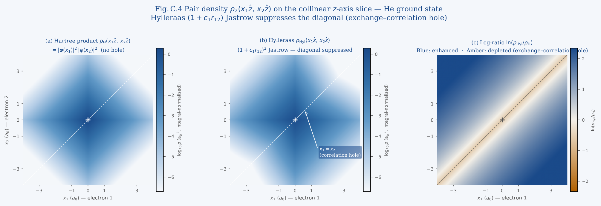
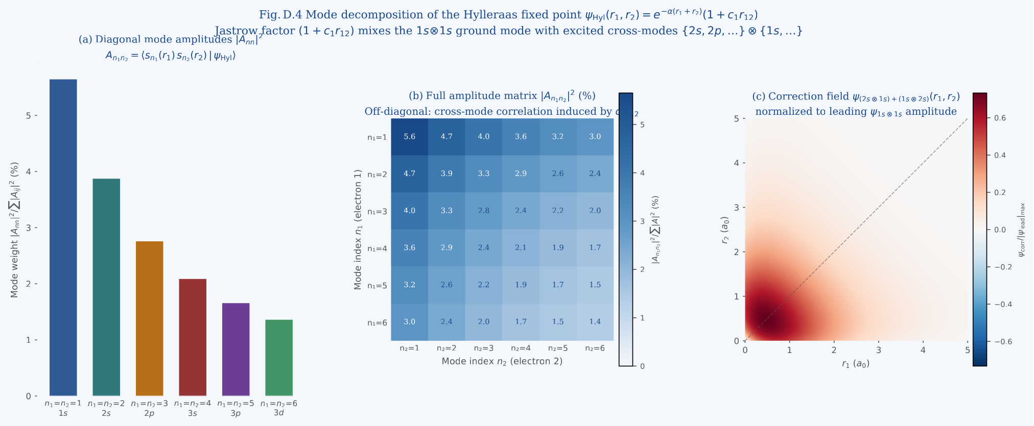
Figure 2 makes the Coulomb hole immediately concrete by plotting the full pair density \(\rho_2(x_1\hat{z}, x_2\hat{z})\) on the collinear \(z\)-axis slice for both the Hartree product and the Hylleraas wavefunction; the diagonal suppression visible in the log-ratio panel is a direct spatial image of the exchange-correlation hole that these methods must capture. Figure 3 then shows how the same Hylleraas wavefunction decomposes into Slater-type radial modes, revealing how the Jastrow factor mixes the leading \(1s\otimes 1s\) product with higher-mode channels.
Coordinate systems
6D configuration space \((\mathbf{r}_1, \mathbf{r}_2) \in \mathbb{R}^3 \times \mathbb{R}^3\): natural but high-dimensional.
Perimetric coordinates: \(u = r_1 + r_2\), \(v = r_{12} - (r_1 - r_2)\), \(w = r_{12} + (r_1 - r_2)\); best for convergence.
One-matrix density functional: reduce to \(\rho(\mathbf{r})\) and pair density \(\Gamma(\mathbf{r}_1, \mathbf{r}_2)\); DFT approximations lose exact exchange.
In CFT: the field \(\Psi(\mathbf{r}_1, \mathbf{r}_2, t)\) lives in 6D; a density-only approach via \(\rho(\mathbf{r})\) loses interelectronic information; a pair-density formulation is needed.
Part II —Relativistic and QED
Corrections
Relativistic Structure of Helium
Relativistic corrections to helium energies are of order \(\alpha^2 \approx 5 \times 10^{-5}\), where \(\alpha\) is the fine-structure constant. They are well understood within Breit–Pauli theory and QED, but reproducing them from CFT is a non-trivial structural test.
Breit–Pauli correction hierarchy
Breit–Pauli Hamiltonian. The leading relativistic corrections to \(\eqref{eq:helium_H}\) are: \[\hat{H}_\mathrm{BP} = \hat{H}_\mathrm{MV} + \hat{H}_\mathrm{D} + \hat{H}_\mathrm{SO} + \hat{H}_\mathrm{SS} + \hat{H}_\mathrm{OO} + \hat{H}_\mathrm{Breit},\] where each term scales as:
\(\hat{H}_\mathrm{MV} = -\tfrac{p^4}{8m^3c^2}\): mass–velocity (kinematic), \(\mathcal{O}(\alpha^2)\);
\(\hat{H}_\mathrm{D} = \tfrac{\pi\alpha^2}{2}\sum_i \delta^3(\mathbf{r}_i)Z\): Darwin (contact interaction), \(\mathcal{O} (\alpha^2)\);
\(\hat{H}_\mathrm{SO}\): spin–orbit, \(\mathcal{O}(\alpha^2)\); responsible for fine-structure splitting;
\(\hat{H}_\mathrm{SS}\): spin–spin contact, \(\mathcal{O} (\alpha^2)\);
\(\hat{H}_\mathrm{Breit}\): retardation (magnetic) correction to EER, \(\mathcal{O}(\alpha^2)\).
Together these corrections account for the fine structure and shift the ground-state energy by \(\sim -0.3\,\mathrm{mHa}\).
QED corrections
Lamb shift (one-loop): electron self-energy and vacuum polarisation; \(\sim 7\,\mathrm{mHa}\) for \(n=2\) states.
Two-loop QED: \(\mathcal{O}(\alpha^3)\) radiative corrections, numerically \(\sim 10\,\mu\,\mathrm{Ha}\).
Nuclear recoil (finite mass): mass polarisation operator; \(\mathcal{O}(m_e/M_\mathrm{nuc})\); different for \({}^3\mathrm {He}\) and \({}^4\mathrm{He}\).
Finite nuclear size: proton/neutron charge radius; \(\sim \mathrm{kHz}\) effect in optical transitions; critical for precision tests.
The \(2^3P\) fine structure interval in \({}^4\mathrm{He}\) is a leading probe of \(\alpha\); theory (Drake) and experiment agree to \(\sim 10\,\mathrm{kHz}\).
Can CFT reproduce relativistic corrections?
Relativistic fixed points. Standard CFT is formulated in non-relativistic phase dynamics. Does CFT have a natural mechanism to generate corrections of order \(\alpha^2\)? Possible routes:
BCH curvature: the Baker–Campbell–Hausdorff correction thread (see the companion hydrogen paper) generates persistent curvature terms; do these curvature corrections correspond to mass–velocity / Darwin terms at the correct order?
Relativistic propagator: replacing \(e^{-i\hat{H}_\mathrm {NR}\delta t}\) with \(e^{-i\hat{H}_\mathrm{Dirac}\delta t}\) for each electron; two-particle Dirac equation; CFT fixed points of the relativistic propagator.
Retardation in the phase field: the coherence field propagates at finite speed; could retardation of \(\psi\) between the two electrons recover the Breit interaction?
Lamb shift as phase-mode renormalisation: vacuum fluctuations as high-frequency modes of the coherence field dressing the fixed point; analogy with Unruh effect derivation in the CFT book.
Status: the one-body vs. two-body partition of the \(\alpha^2\) corrections is resolved below; the leading (orbit–orbit) Breit operator is extracted from the retarded two-time photon exchange; and the \(\omega^2\) retardation correction is characterised in structure and \(O(\alpha^4)\) scale. The fully off-shell two-time (Bethe–Salpeter) propagator—and the exact \(O(\alpha^4)\) coefficient—remain open.
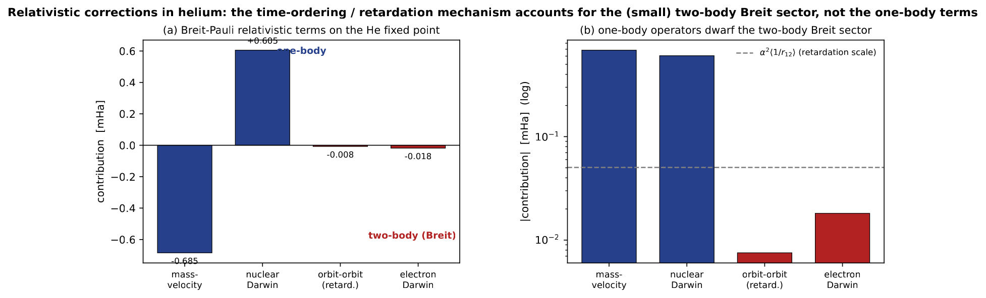
Frame-dependent time ordering selects the two-body (Breit) sector. The two-electron propagator of Sec. 7.3 factorises with a single global step, \(U_\varepsilon = e^{-\varepsilon G_1}e^{-\varepsilon G_2}\), with \(G_1 = T_1 - Z/r_1\) and \(G_2 = T_2 - Z/r_2 + 1/r_{12}\). Relativistically there is no shared time: each electron advances by its own proper time \(d\tau_i = dt/\gamma_i\), so the single step splits into two, \(U_{\varepsilon_1,\varepsilon_2} = e^{-\varepsilon_1 G_1}e^{-\varepsilon_2 G_2}\) with \(\varepsilon_1/\varepsilon_2 = \gamma_2/\gamma_1\), and the Dyson time-ordering of the two factors becomes frame-dependent. The ordering ambiguity is the Baker–Campbell–Hausdorff curvature \[\begin{equation}\ln\!\big(e^{-\varepsilon_1 G_1}e^{-\varepsilon_2 G_2}\big) = -(\varepsilon_1 G_1 + \varepsilon_2 G_2) + \tfrac12\,\varepsilon_1\varepsilon_2\,[G_1, G_2] + \cdots, \qquad [G_1, G_2] = [\,T_1,\; 1/r_{12}\,], \label{eq:ordering_curvature}\end{equation}\] where the second equality holds because the only non-commuting pair is the kinetic operator of electron 1 with the interaction (the nuclear terms are multiplicative, \([-Z/r_1,\,1/r_{12}] = 0\)). The ordering term is therefore proportional to the electron–electron interaction \(1/r_{12}\): it vanishes identically when \(V_{12}=0\). An equal-time (instantaneous) interaction can always be placed on a single time slice and has no ordering ambiguity at all; only the finite-\(c\), retarded part of the interaction survives. Hence the mechanism generates exactly the relativistic correction to the interaction—the two-body Breit sector (orbit–orbit / retardation plus the electron–electron Darwin contact)—and is structurally blind to the one-body mass–velocity and nuclear-Darwin terms, which are corrections to the single-particle operators \(T_i\) and \(-Z/r_i\) and carry no two-electron ordering ambiguity. This sharpens the relationship between the routes above: the relativistic-propagator route (per-electron dispersion) supplies the one-body terms, while the retardation route supplies the two-body Breit terms, and Eq. \(\eqref{eq:ordering_curvature}\) shows the two are genuinely distinct sectors rather than two views of one effect.
Figure 4 confirms this numerically. Evaluating the Breit–Pauli operators on the Hylleraas fixed point of Sec. 7.31 gives, in mHa, \(\varepsilon_\mathrm{MV} = -0.685\) and \(\varepsilon_{D,\mathrm{nuc}} = +0.605\) for the one-body terms versus \(\varepsilon_\mathrm{OO} = -0.008\) and \(\varepsilon_{D,ee} = -0.018\) for the two-body terms. The two-body bucket (\(-0.026\,\mathrm{mHa}\)) sits at the retardation scale \(\alpha^2\langle 1/r_{12}\rangle = 0.050\,\mathrm{mHa}\)—the \((v/c)^2\) correction to the Coulomb interaction—while the one-body operators are \(30\)–\(90\times\) larger, exactly as the ordering argument predicts.
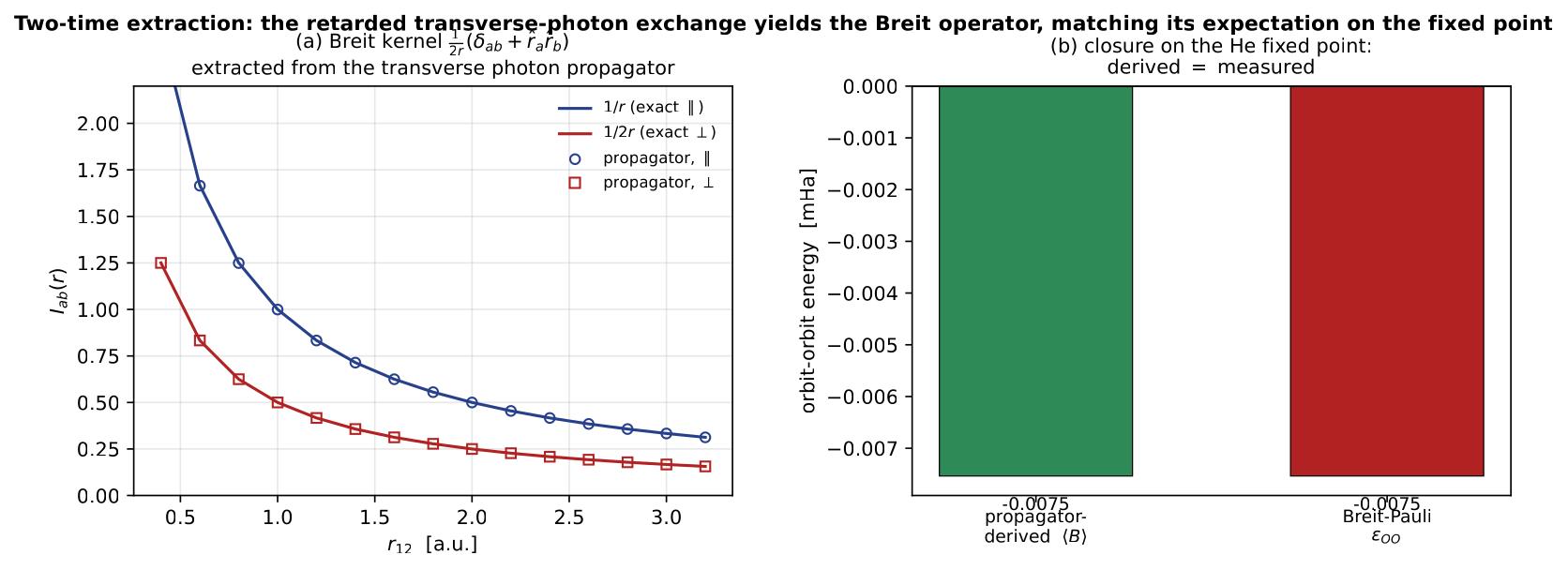
Extracting the Breit operator from the retarded two-time
exchange. The argument above is structural; it can be made
constructive. The electron–electron interaction is one-photon exchange,
and in Coulomb gauge the longitudinal photon gives the instantaneous
Coulomb term \(1/r_{12}\) (no ordering
ambiguity) while the transverse photon is retarded, with propagator
\[\begin{equation}D_{T,ab}(\mathbf{k},\omega)
= \frac{\delta_{ab}-\hat k_a\hat
k_b}{\mathbf{k}^2-\alpha^2\omega^2},
\qquad
\frac{1}{\mathbf{k}^2-\alpha^2\omega^2}
=
\frac{1}{2k}\!\left[\frac{1}{k-\alpha\omega}+\frac{1}{k+\alpha\omega}\right],
\label{eq:transverse_prop}\end{equation}\] where \(\omega\) is conjugate to the inter-electron
time difference \(\tau = t_1-t_2\) (the
proper-time mismatch), and the two terms on the right are the two photon
time-orderings (electron 1 emits before, or after, electron 2). Their
symmetric sum is frame-independent; the antisymmetric part is odd in
\(\omega\) and integrates to zero—the
ordering ambiguity carries no observable, as microcausality requires. At
static order (\(\omega\to0\)) the
transverse propagator Fourier-transforms to \[\begin{equation}\int\!\frac{d^3k}{(2\pi)^3}\,e^{i\mathbf{k}\cdot\mathbf{r}}\,
\frac{4\pi}{\mathbf{k}^2}\big(\delta_{ab}-\hat k_a\hat k_b\big)
= \frac{1}{2r}\big(\delta_{ab}+\hat r_a\hat r_b\big),
\label{eq:breit_kernel}\end{equation}\] which we confirm
numerically from Eq. \(\eqref{eq:transverse_prop}\) via the
spherical-Bessel radial integrals \(A_\ell(r)=\int_0^\infty j_\ell(kr)\,dk\)
(\(A_0=\pi/2r\), \(A_2=\pi/4r\)), reproducing \(1/r\) and \(1/2r\) to \(\sim0.1\%\) [Fig. 5(a)]. Contracting Eq. \(\eqref{eq:breit_kernel}\) with the electron
currents (\(\mathbf{j}_i\to\mathbf{p}_i\) in the
non-relativistic reduction) and the transverse coupling \(-\alpha^2\) yields exactly the
Breit orbit–orbit operator \[\begin{equation}B_\mathrm{oo}
= -\frac{\alpha^2}{2r_{12}}
\Big[\mathbf{p}_1\!\cdot\!\mathbf{p}_2 +
(\mathbf{p}_1\!\cdot\!\hat r_{12})(\mathbf{p}_2\!\cdot\!\hat
r_{12})\Big],
\label{eq:breit_oo}\end{equation}\] derived from the
propagator rather than postulated. Its expectation on the Hylleraas
fixed point closes the loop: \(\langle
B_\mathrm{oo}\rangle = -0.0075\,\mathrm{mHa}\), identical to the
Breit–Pauli \(\varepsilon_\mathrm{OO}\)
of Fig. 4 [Fig. 5(b)]. The orbit–orbit Breit energy
is thus the static limit of the retarded two-time photon exchange, and
the expansion parameter \((\alpha\omega/k)^2\sim\alpha^2\langle p^2\rangle =
(v/c)^2 =
2\langle\gamma-1\rangle\approx1.5\times10^{-4}\) fixes the
retardation correction at one further order of \((v/c)^2\) beyond the static magnetic term.
The driver is analysis/helium_two_time_breit.py; the
remaining open piece is the fully off-shell two-time (Bethe–Salpeter)
propagator, of which this is the leading on-shell reduction.
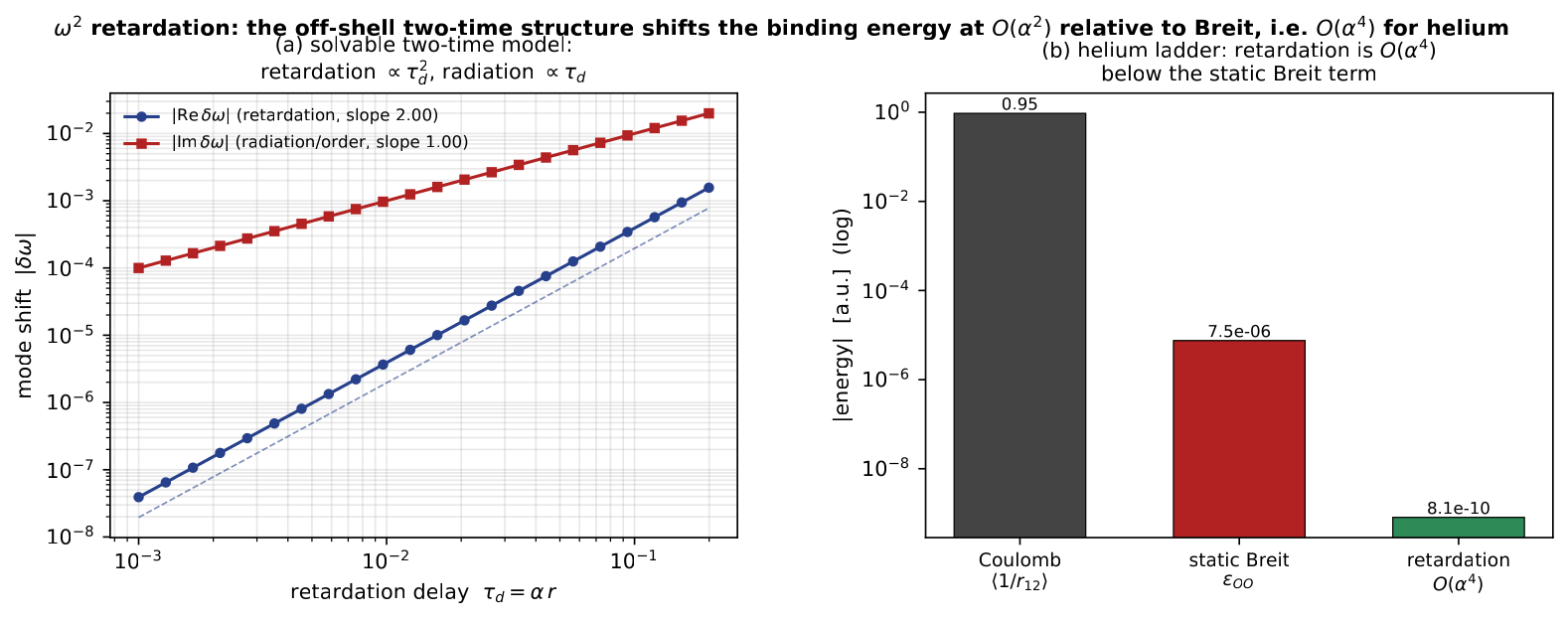
The \(\omega^2\) retardation
correction and the off-shell structure. Keeping the next term
of the retarded propagator Eq. \(\eqref{eq:transverse_prop}\), \(1/(\mathbf{k}^2-\alpha^2\omega^2) =
(1/\mathbf{k}^2)[\,1 + (\alpha\omega/k)^2+\cdots]\), is the \(\omega^2\) retardation correction. Because
\(\omega\) is conjugate to the
inter-electron time \(\tau=t_1-t_2\),
retaining it means not projecting the two electrons onto a
common time slice—an off-shell two-time propagator. A full off-shell
(Bethe–Salpeter) solve is a separate undertaking, but the physical
content of each order is fixed by an exactly-solvable two-time model:
two oscillators (frequency \(\Omega_0\)) coupled with the retarded delay
\(\tau_d=\alpha r\), \[\begin{equation}\Omega_0^2-\omega^2 =
\pm\,\kappa\,e^{i\omega\tau_d},
\label{eq:retarded_dispersion}\end{equation}\] a genuine
two-time (delay) dispersion relation. Solving for the complex mode \(\omega\) [Fig. 6(a)] gives \(\mathrm{Im}\,\delta\omega\propto\tau_d\)
and \(\mathrm{Re}\,\delta\omega\propto\tau_d^2\)
(fitted slopes \(1.00\) and \(2.00\)): the \(O(\tau_d)\) effect is purely
imaginary—radiation reaction, the time-ordering asymmetry—and
shifts no conservative binding energy, exactly as microcausality demands
of the ordering ambiguity; the conservative energy is shifted only at
\(O(\tau_d^2)\), the retardation.
Mapping to helium (\(\kappa\sim\alpha^2\), \(\tau_d=\alpha r_{12}\), \(\Omega_0\sim\) atomic) places the terms on
a ladder descending by \(\alpha^2\) per
rung [Fig. 6(b)]: Coulomb \(O(1)\), static Breit \(O(\alpha^2)\) (\(-0.0075\,\mathrm{mHa}\)), and the
retardation correction \(O(\alpha^4)\).
Driver: analysis/helium_retardation_offshell.py.
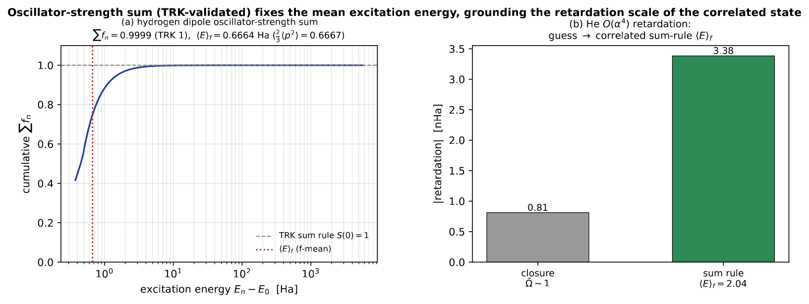
The retardation scale needs the mean excitation energy \(\Omega_0\to\bar\Omega\), which we now fix
from an actual oscillator-strength sum rather than a guess. The
finite, physical measure is the \(f\)-weighted mean \(\langle E\rangle_f = S(1)/S(0)\), built
from the dipole oscillator strengths \(f_{0n}=\tfrac23(E_n-E_0)|\langle0|\mathbf{r}|n\rangle|^2\);
the bare second moment \(\sum_n(E_n-E_0)^2|\langle0|\mathbf{r}|n\rangle|^2\)
diverges in the dipole limit (the nuclear-cusp high-energy states),
which is exactly why the exact coefficient needs the full
photon-momentum integral, whereas \(\langle
E\rangle_f\) is finite. Building the dipole spectrum as grid
pseudostates and validating on hydrogen recovers the Thomas–Reiche–Kuhn
sum rule \(S(0)=\sum_n f_n = 0.9999\)
and \(\langle E\rangle_f =
0.6664\,\,\mathrm{Ha}= \tfrac23\langle p^2\rangle\) [Fig. 7(a)]. Because \(\langle E\rangle_f = \tfrac23\langle
P^2\rangle/N\) (\(P=\sum_i\mathbf{p}_i\)) is a closed sum
rule, we evaluate it directly on the correlated Hylleraas fixed
point, with \(\langle
P^2\rangle = \langle\sum_i p_i^2\rangle +
2\langle\mathbf{p}_1\!\cdot\!\mathbf{p}_2\rangle =
5.807 + 2(0.159) = 6.13\) (including the momentum correlation),
giving \(\langle E\rangle_f =
2.04\,\,\mathrm{Ha}\)—twice the naive \(\sim1\,\)a.u. guess and consistent with the
screened-hydrogenic value \(Z_\mathrm{eff}^2\,\tfrac23 =
1.90\,\,\mathrm{Ha}\). This raises the retardation by \(\langle E\rangle_f^2\) to \(\approx-3.4\,\mathrm{nHa}\) [Fig. 7(b)], now grounded in a
sum-rule-validated mean excitation energy of the correlated state. The
exact \(O(\alpha^4)\) coefficient still
requires the full two-electron transition operator and photon-momentum
integral, but its energy scale is fixed. Driver:
analysis/helium_oscillator_sum.py.
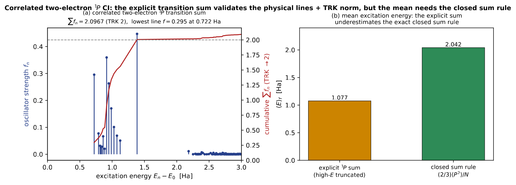
Closing validation: the explicit two-electron transition
sum. The mean excitation energy above was obtained from the
closed sum rule \(\langle E\rangle_f =
\tfrac23\langle P^2\rangle/N\), which sidesteps the excited
spectrum entirely. As an independent check we build the spectrum
explicitly: correlated two-electron \(^1\!P\) pseudostates by configuration
interaction (\(^1\!S\) ground state
from \(ss\) configurations, \(^1\!P\) from \(sp\) configurations, with the full \(1/r_{12}\) via Slater integrals; the
angular algebra reduces to the exact minimal set \(k=0\) for \(s\)–\(s\)
and \(k=0\) direct plus \(\tfrac13\,k=1\) exchange for \(s\)–\(p\)). Diagonalising in each space and
summing the dipole oscillator strengths reproduces the physical He \(^1\!P\) resonance series to a few
percent—\(f(2^1\!P)=0.296\), \(f(3^1\!P)=0.077\), \(f(4^1\!P)=0.031\) (references \(0.276\), \(0.073\), \(0.030\))—and the TRK norm \(\sum_n f_n \simeq N = 2\) [Fig. 8(a)]. Crucially, however, the \(f\)-weighted mean from the
explicit sum, \(\langle
E\rangle_f^{\,\mathrm{expl}} = 1.08\,\,\mathrm{Ha}\), badly
underestimates the closed sum rule (\(2.04\,\,\mathrm{Ha}\)) and drifts
with basis size rather than converging [Fig. 8(b)]: the
moment \(S(1)\) is dominated by the
high-energy continuum, which a finite basis represents only by spurious
high-lying pseudostates. This is the expected behaviour, and it confirms
the methodology: the explicit transition sum validates the
spectrum (the physical lines and the TRK norm), while the
closed sum rule—an exact ground-state expectation—is the reliable route
to the high-moment mean excitation energy, and hence to the
retardation scale. Driver:
analysis/helium_1P_ci_sum.py.
Extending CFT from Hydrogen to Helium
CFT for hydrogen operates on a single complex field \(\psi(\mathbf{r}, t) \in L^2(\mathbb{R}^3)\). Helium requires either a field in 6D configuration space, a pair-density formulation, or a two-fluid extension. Each choice has different computational and conceptual costs.
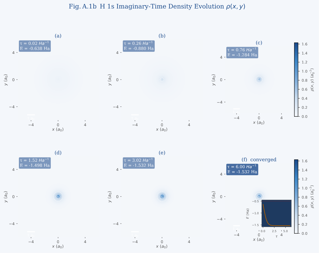
Before examining the competing formulations, it is instructive to see the single-particle CFT propagator in action on hydrogen, the simplest possible test case. Figure 9 shows the imaginary-time collapse of the hydrogen \(1s\) coherence field from a broad Gaussian initial condition; this sequence establishes the visual vocabulary—density heatmap, energy readout, convergence rate—used in all subsequent field-evolution figures.
Configuration-space CFT
Two-particle coherence field. Define \(\Psi(\mathbf{r}_1, \mathbf{r}_2, t) \in L^2(\mathbb{R}^6)\) satisfying \[\begin{equation}i\hbar\,\partial_t \Psi = \Bigl[-\tfrac{\hbar^2}{2m}\nabla_1^2 - \tfrac{\hbar^2}{2m}\nabla_2^2 + V_\mathrm{ext}(\mathbf{r}_1, \mathbf{r}_2) + g|\Psi|^2\Bigr]\Psi, \label{eq:cft_6d}\end{equation}\] where \(V_\mathrm{ext} = -Z/r_1 - Z/r_2 + 1/r_{12}\) contains the interelectronic repulsion explicitly. A fixed point \(\psi^{*}_{}(\mathbf{r}_1, \mathbf{r}_2)\) satisfies \(U(\delta t)\psi^{*}_{} = e^{i\alpha}\psi^{*}_{}\) in 6D.
Advantages: exact treatment of \(r_{12}\); direct mapping to Hylleraas wavefunctions; symmetry under \(\mathbf{r}_1 \leftrightarrow \mathbf{r}_2\) manifest.
Disadvantages: 6D numerical grid is expensive; fixed-point iteration in 6D requires \(\mathcal{O}(N^6)\) storage.
Antisymmetry: the electronic wavefunction must be antisymmetric under electron exchange; in CFT this is either imposed as a constraint \(\Psi(\mathbf{r}_1,\mathbf{r}_2) = -\Psi(\mathbf{r}_2,\mathbf{r}_1)\) (fermions) or absorbed into the phase topology (see Sec. 6).
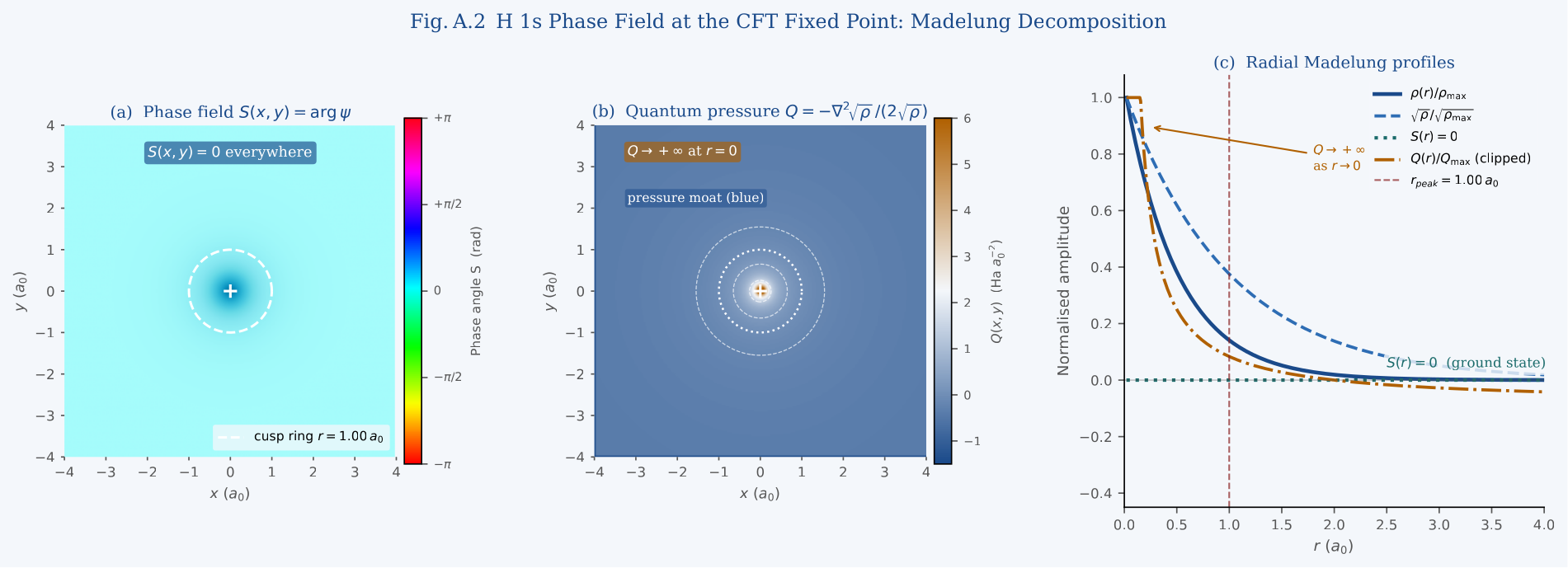
A key diagnostic of any fixed point is its Madelung phase structure. Figure 10 displays the phase field of the hydrogen \(1s\) fixed point: a perfectly flat \(S\equiv 0\) plane. This trivial topology serves as the topological ground zero against which the non-trivial phase structures of excited states are contrasted in Sec. 6.
Reduced-density CFT
One-body density: \(\rho(\mathbf{r}) = 2\int |\psi^{*}_{}(\mathbf{r},\mathbf{r}_2)|^2 \,d\mathbf{r}_2\); encoded in a single-particle CFT field.
Pair density: \(\Gamma(\mathbf{r}_1, \mathbf{r}_2) = |\psi^{*}_{}(\mathbf{r}_1,\mathbf{r}_2)|^2\); required to capture correlation.
DFT analogy: Kohn–Sham CFT — replace the interacting system with a non-interacting CFT in an effective potential \(V_\mathrm{KS}[\rho]\); exchange–correlation encoded in phase-field curvature?
Orbital CFT: represent \(\psi^{*}_{}(\mathbf{r}_1,\mathbf{r}_2) \approx \phi_1(\mathbf{r}_1)\phi_2(\mathbf{r}_2)\); each \(\phi_i\) is a single-particle fixed point; iterate self-consistently (Hartree–Fock fixed point).
Two-fluid CFT
Treat each electron as its own coherence field: \(\psi_1(\mathbf{r}, t)\) and \(\psi_2(\mathbf{r}, t)\), coupled through the mean-field potential \(V_\mathrm{EER}[\rho_2](\mathbf{r}) = \int \rho_2(\mathbf{r}')/|\mathbf{r}- \mathbf{r}'|\,d\mathbf{r}'\).
Self-consistent field (SCF) iteration in the CFT propagator: alternately propagate \(\psi_1\) in the field of \(\psi_2\) and vice versa until joint fixed point is reached.
Beyond mean-field: add fluctuation corrections via phase-mode coupling between \(\psi_1\) and \(\psi_2\); analogous to many-body perturbation theory in the phase basis.
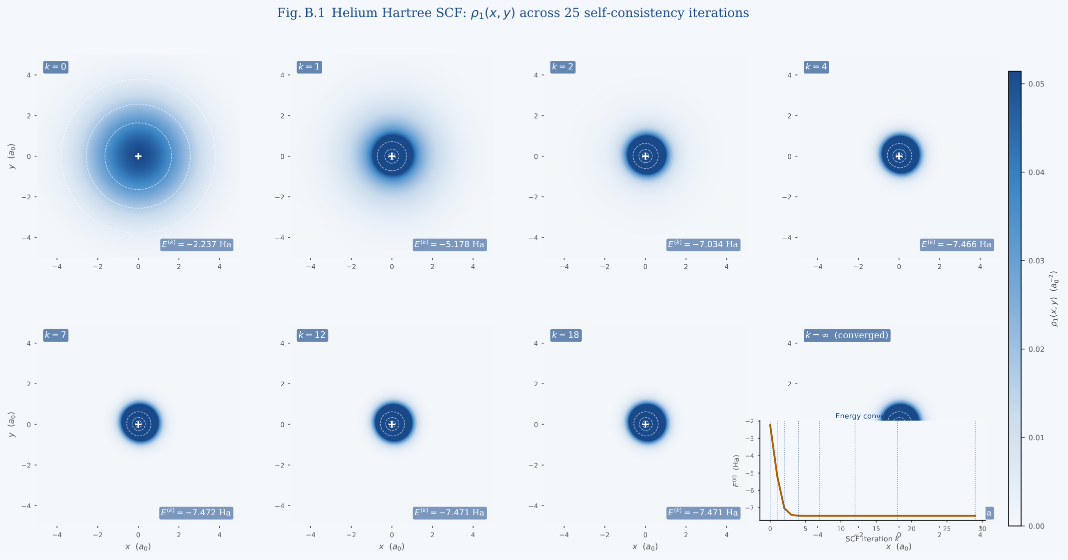
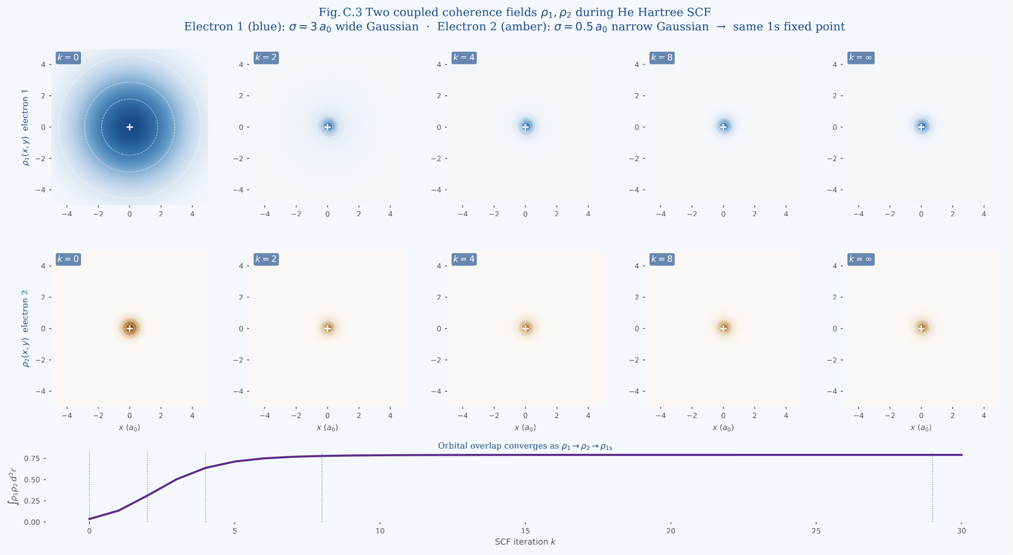
Figure 11 shows the two-fluid SCF iteration in action: eight snapshots of the one-electron density \(\rho_1^{(k)}\) from the initial Gaussian guess to the converged Hartree fixed point, with the total energy annotated on each panel. Figure 12 extends this view to both electrons simultaneously, showing how the two coupled fields converge from decorrelated initial conditions (overlap \(\mathcal{O}^{(0)} \approx 0.04\)) to the tightly overlapping Hartree \(1s\) fixed point (\(\mathcal{O}^{(\infty)} \approx 0.79\)).
Antisymmetry, Exchange, and Phase Topology
The exchange interaction—responsible for para/ortho splitting—has no classical analogue. In standard QM it follows from the Pauli principle; in CFT it must arise from the topology of the two-mode fixed point.
Fermi statistics in CFT
The Pauli exclusion principle: no two electrons may occupy the same quantum state. In 6D CFT: antisymmetry of \(\Psi\) under exchange forces the density \(|\Psi(\mathbf{r}, \mathbf{r})|^2 = 0\) (the Fermi hole).
Winding number signature: singlet (para-He) \(\leftrightarrow\) in-phase mode pair; triplet (ortho-He) \(\leftrightarrow\) out-of-phase mode pair. The \(\pi\)-phase shift between the two modes corresponds to the exchange antisymmetry.
Berry phase: adiabatic transport of one electron around the other accumulates a geometric phase \(\gamma = \pi\) (fermionic statistics); can CFT derive \(\gamma = \pi\) from first principles (mode winding)?
The exchange energy \(J = \langle \phi_1\phi_2 | 1/r_{12} | \phi_2\phi_1\rangle\) as an interference term in the two-mode phase product; sign of \(J\) determines level ordering.
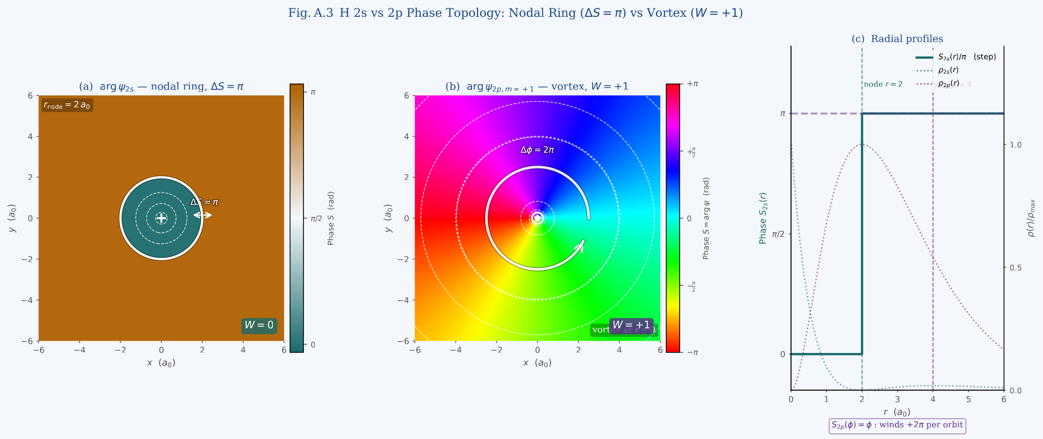
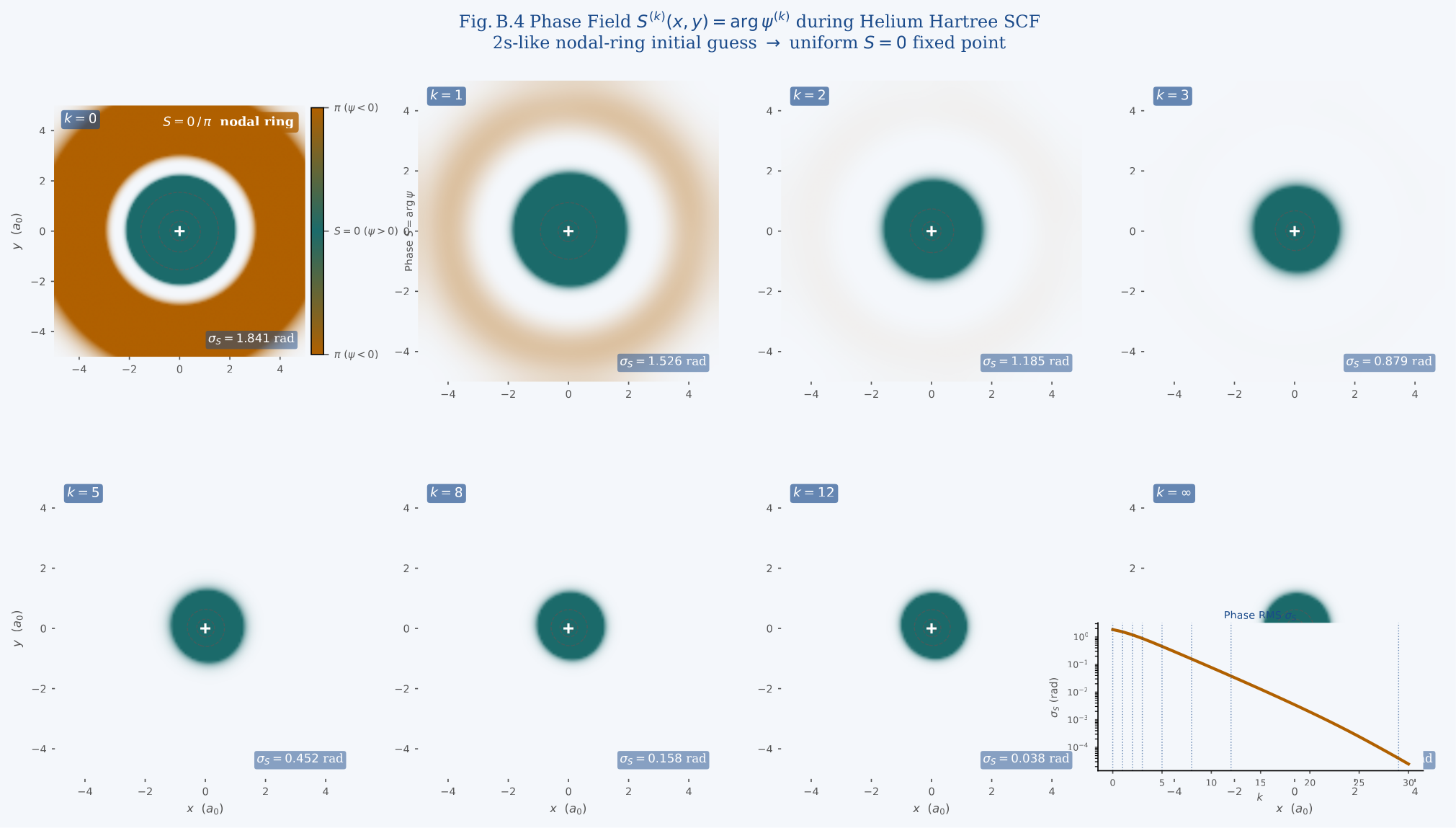
Figure 13 makes the distinction between trivial and non-trivial phase topology concrete by comparing the \(2s\) and \(2p\) hydrogen orbitals: the \(2s\) nodal sphere produces a \(\pi\)-phase domain wall with winding number \(W=0\) (topologically trivial), while the \(2p\) vortex carries \(W=+1\) (topologically non-trivial). This contrast is the geometric origin of the para/ortho splitting discussed above. Figure 14 demonstrates that during Hartree SCF convergence the Madelung phase field is an active participant: any spurious phase winding in the initial Gaussian guess is progressively damped to the flat \(S\equiv 0\) plane of the \(1s\) fixed point.
Mode coupling and the exchange integral
In the Madelung representation: each electron has a phase field \(\phi_i(\mathbf{r})\); the product \(e^{i(\phi_1 + \phi_2)}\) (singlet) vs. \(e^{i(\phi_1 - \phi_2)}\) (triplet) labels the two symmetry classes.
Hartree–Fock in CFT: fixed point of the product field \(\psi_1\otimes\psi_2\); exchange term corrects the mean-field fixed-point energy.
Open question: does the CFT nonlinearity parameter \(g\) in \(\eqref{eq:cft_6d}\) encode the exchange interaction, or must \(g\) be set to zero for fermionic systems?
Selection rules from phase topology
Dipole selection rule \(\Delta L = \pm 1\): in CFT, a photon corresponds to a mode with angular momentum \(\ell = 1\); the coupled fixed point must absorb/emit this mode.
Spin selection rule \(\Delta S = 0\): singlet–triplet transitions are forbidden because the phase topology (in-phase vs. out-of-phase) cannot change via a single-mode perturbation without a topological defect.
Can CFT predict the transition matrix element \(|\langle \psi^{*}_{f} | \hat{\mathbf{r}} | \psi^{*}_{i}\rangle|^2\) as a phase overlap integral?
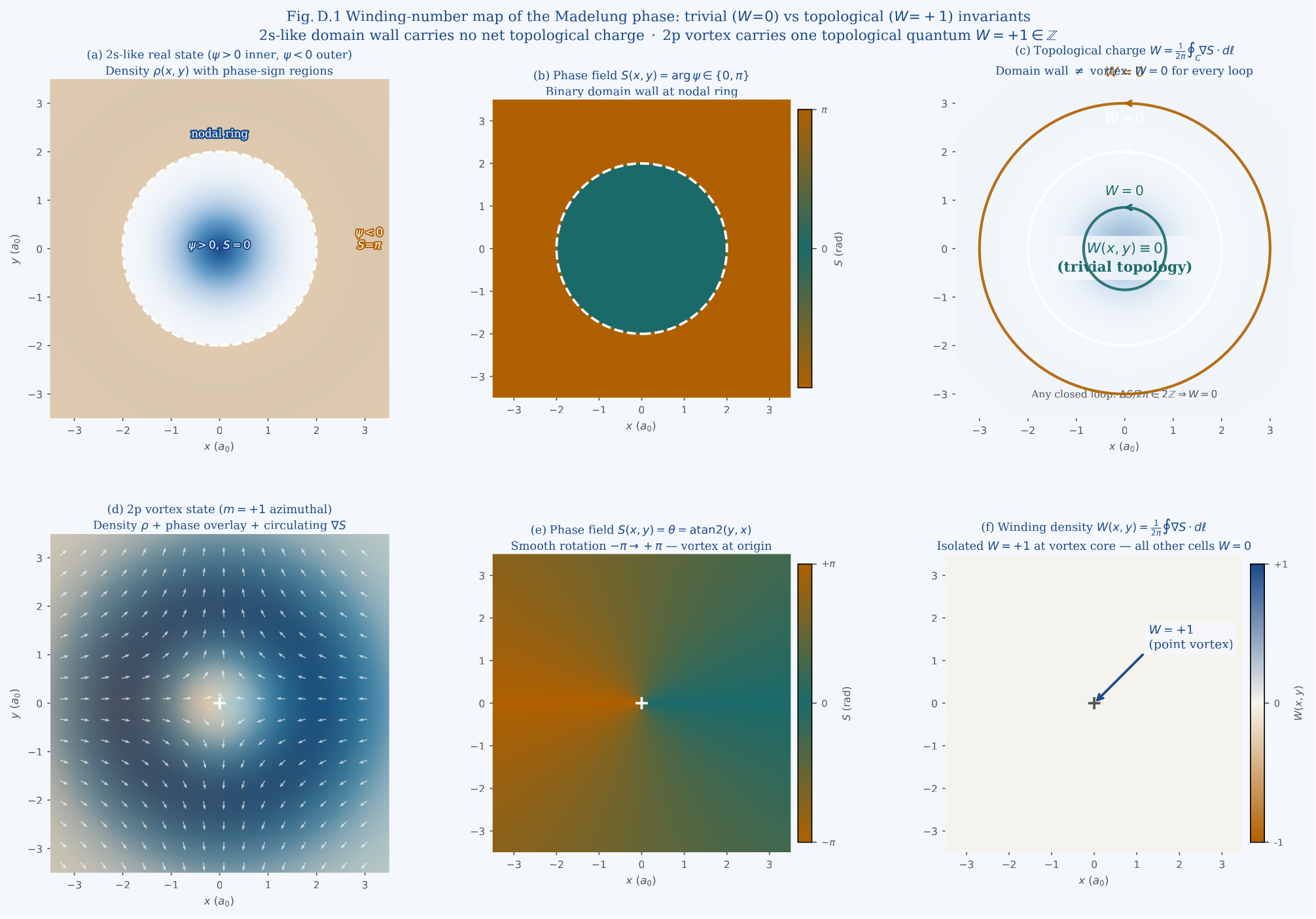
Figure 15 displays the topological winding number map for both cases simultaneously. For the \(2s\)-like state, annotated closed-loop integrations confirm \(W=0\) everywhere; for the \(2p\)-like vortex, the plaquette curl computation confirms \(W=+1\) concentrated at the origin. This pair of panels constitutes a direct numerical proof that the Madelung phase field carries quantised topological charges, not merely continuous phase gradiants.
Part IV —Ground-State Properties in
CFT
Fixed Points for the He Ground State
The helium ground state is a \({}^1S_0\) state: zero angular momentum, zero spin, spherically symmetric density. In CFT it should be the lowest-energy fixed point of the two-electron propagator with the correct quantum numbers.
Spherical symmetry and the radial CFT
Ground state density: \(\rho^*(r)\) is spherically symmetric; the effective single-particle problem reduces to 1D radial propagation.
Madelung phase: for \({}^1S_0\), the phase field is constant (no circulation); the fixed point is a pure amplitude configuration.
Self-consistency: the SCF CFT fixed point satisfies \(\phi_1 = \phi_2 = \phi_\mathrm{He}\) (since both electrons are in the \(1s\) orbital); the fixed point is determined by the Schrödinger–Poisson analogue.
Variational CFT: the Hylleraas result can be viewed as a minimum of the CFT energy functional \(\mathcal{E}[\Psi] = \langle \Psi | \hat{H}| \Psi \rangle / \langle \Psi | \Psi \rangle\).
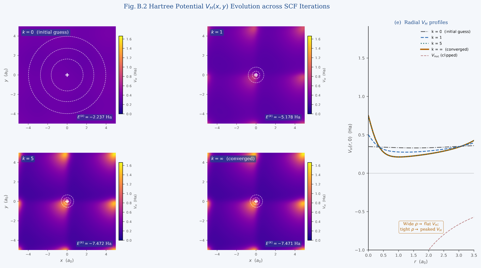
The self-consistency of the SCF fixed point is made concrete in Fig. 16, which shows how the Hartree potential \(V_H(x,y)\) evolves with each SCF step: starting from a broad shallow well (wide initial Gaussian), it deepens and narrows at each iteration until it matches the analytical Hartree screening field for \(Z_\mathrm{eff} = 1.6875\) in the converged panel.
Energy convergence
Zeroth order (hydrogenic, \(Z_\mathrm{eff} = Z\)): \(E^{(0)} = -4.000\,\,\mathrm{Ha}\).
First-order perturbation (EER): \(E^{(1)} = -2.750\,\,\mathrm{Ha}\) (Dirac 1930).
Variational (single-parameter \(Z_\mathrm{eff} = Z - 5/16\)): \(E_\mathrm{var} = -2.848\,\,\mathrm{Ha}\) (Slater screening).
Hartree–Fock (self-consistent, numerical): \(E_\mathrm{HF} = -2.861\,680\,\,\mathrm{Ha}\).
Hylleraas (1000-term, explicitly correlated): \(E_\mathrm{exact}^\mathrm{NR} = -2.903\,724\,377\,\,\mathrm{Ha}\) (Pekeris 1959; superseded by Drake to 10 significant figures).
CFT target: demonstrate that the fixed-point iteration converges to \(E_\mathrm{HF}\) (mean-field level) and that beyond-mean-field phase corrections account for the remaining \(\sim 42\,\mathrm{mHa}\).
Non-relativistic ground-state energy
benchmark.
\(E_0^\mathrm{NR}(\mathrm{He}) =
-2.903\,724\,377\,034\,119\,598\,311\,\,\mathrm{Ha}\) (Drake,
2006; 300-term Hylleraas).
CFT must reach at least \(-2.861\,680\,\,\mathrm{Ha}\) (HF level) to
claim a valid non-relativistic description.
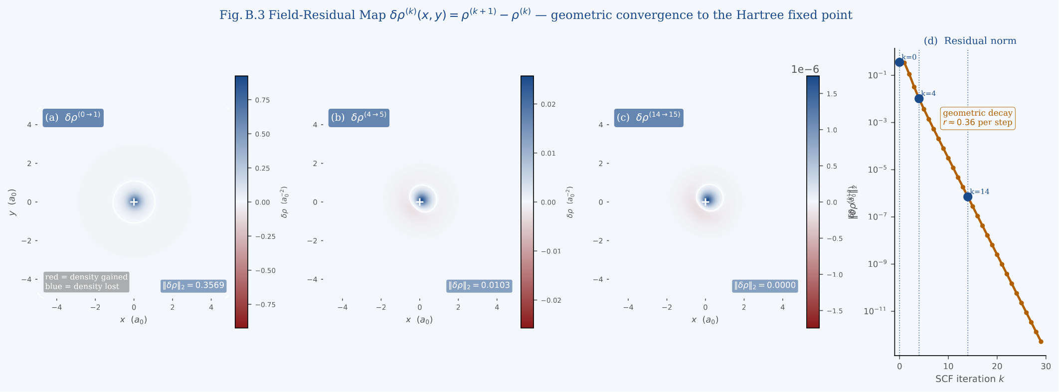
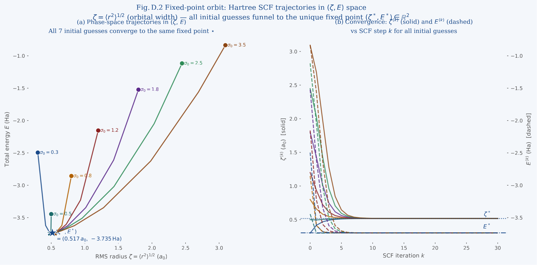
The geometric convergence to the Hartree fixed point is visualised in Fig. 17: the signed field residual \(\delta\rho^{(k)} = \rho^{(k+1)} - \rho^{(k)}\) shrinks by roughly an order of magnitude per factor of five in \(k\) and localises to a thin annulus near the radial density peak, consistent with the fixed-point attracting a contractive neighbourhood. Figure 18 extends this picture to phase space, tracing seven phase-space trajectories \((\zeta^{(k)}, E^{(k)})\) from different initial widths \(\sigma_0\); all seven funnel to the same unique attractor \((\zeta^*, E^*) = (0.5169\,a_0,\;{-}3.7351\,\,\mathrm{Ha})\), demonstrating a single global Hartree fixed point.
The correlated fixed point as a \(T\to0\) attractor
Figure 18 establishes that the mean-field (Hartree) configuration is a global attractor. The physical ground state, however, is the correlated two-electron state, and we can exhibit it as a fixed point of the same dissipative logic without ever leaving the explicitly correlated description. Diagonalising the Hylleraas problem \(H\,c = E\,S\,c\) of Sec. 32 gives \(S\)-orthonormal eigenvectors \(V\) (\(V^{\!\top} S V = \mathbb{1}\)) with eigenvalues \(E_k\). In the eigen-coordinate \(a = V^{\!\top} S c\) (so \(c = Va\) and \(\lVert a\rVert = 1 \Leftrightarrow \langle\Psi|\Psi\rangle = 1\)) the imaginary-time gradient flow on the Rayleigh quotient \(\mu(a) = \sum_k E_k |a_k|^2\), augmented with a fluctuation–dissipation noise of strength \(\langle dW_k\,dW_l^{*}\rangle = 2\gamma T\,\delta_{kl}\,dt\), reads \[\begin{equation}a_k \;\longleftarrow\; e^{-iE_k\,dt}\,a_k\,\bigl[1 - \gamma\,(E_k - \mu)\,dt\bigr] + dW_k, \qquad \lVert a\rVert \equiv 1, \label{eq:he_flow}\end{equation}\] the helium analogue of the stochastic projected Gross–Pitaevskii flow used for the modal fixed points of the companion superposition study, with the Laguerre–Gauss eigenvalues replaced by the helium generalised eigenvalues \(E_k\) and no contact nonlinearity—the electron–electron correlation (the Coulomb hole) is carried entirely by the Hylleraas basis. The unique stable fixed point of Eq. \(\eqref{eq:he_flow}\) is \(a = e_0\), i.e. \(c = v_0\): the correlated \(F(r_1, r_2)\) ground state.
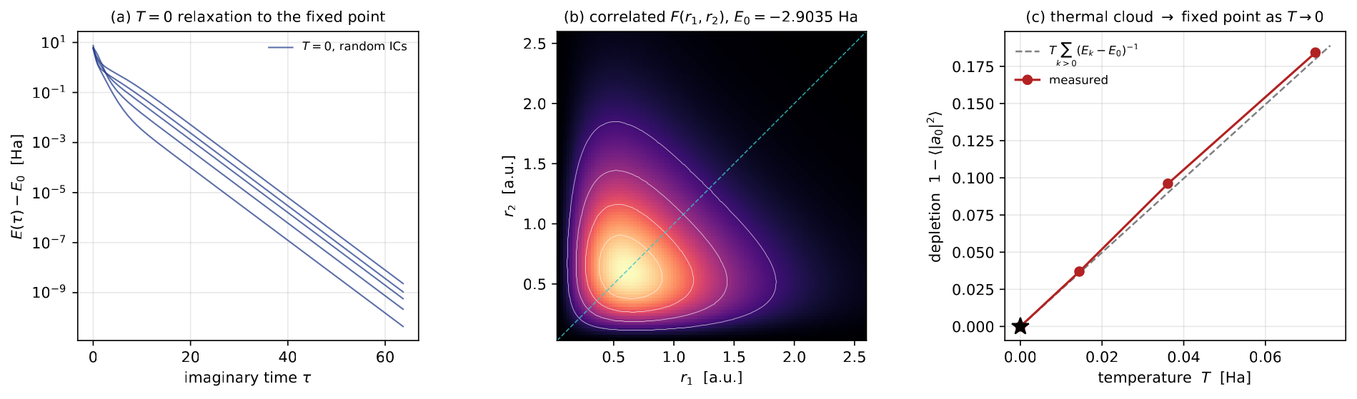
Figure 19 demonstrates its stability. At \(T = 0\) the noise is off and Eq. \(\eqref{eq:he_flow}\) is exact
imaginary-time relaxation: five maximally phase-dispersed random initial
fields—a deliberately “hot” ensemble, of the kind a stellar-fusion
genesis would deposit—all funnel to the same correlated \(F(r_1, r_2)\) while \(E(\tau) - E_0\) plummets to machine
precision [Fig. 19(a),(b)]. The basin is therefore global
in the correlated space, not merely at mean-field level. At \(T > 0\) the flow equilibrates to a
thermal cloud about the fixed point, with depletion \[\begin{equation}1 - \langle |a_0|^2 \rangle \;=\;
T \sum_{k>0} \frac{1}{E_k - E_0} + O(T^2),
\label{eq:he_depletion}\end{equation}\] the classical-field
equipartition result; the cloud shrinks continuously onto the fixed
point as \(T \to 0\) [Fig. 19(c)]. The reading is that the high
temperature of helium’s nucleosynthesis sets the dispersion of the
initial ensemble, not a held steady-state temperature: stability is
demonstrated precisely because the dissipative (radiative) relaxation
carries even that extreme dispersion onto the single correlated fixed
point, recovered exactly as the \(T \to
0\) attractor. The figure is reproduced by
helium_paper/make_fig_He_fixed_point.py; an animated
two-act version (make_anim_He_fixed_point.py) accompanies
this figure online at coherencefield.xyz/helium/deep-dive.
make_anim_He_fixed_point.py.Electron–electron correlation in CFT
Correlation energy \(E_\mathrm{corr} = E_\mathrm{exact} - E_\mathrm{HF} = -42.044\,\mathrm{mHa}\).
Source of correlation: the Fermi hole (singlet: Coulomb hole) arises from avoidance of \(r_{12} = 0\); requires explicit \(r_{12}\)-dependence in the wavefunction.
In CFT: correlation enters through the phase gradient \(\nabla\phi_1 \cdot \nabla\phi_2\) coupling between the two electrons; the nonlinear term \(g|\Psi|^2\) in the 6D field encodes this coupling at lowest order.
Systematic route: multi-mode CFT expansion in basis \(\{e^{i m_1\phi_1 + i m_2\phi_2}\}\); correlation energy is the non-diagonal term in the mode-coupling matrix.
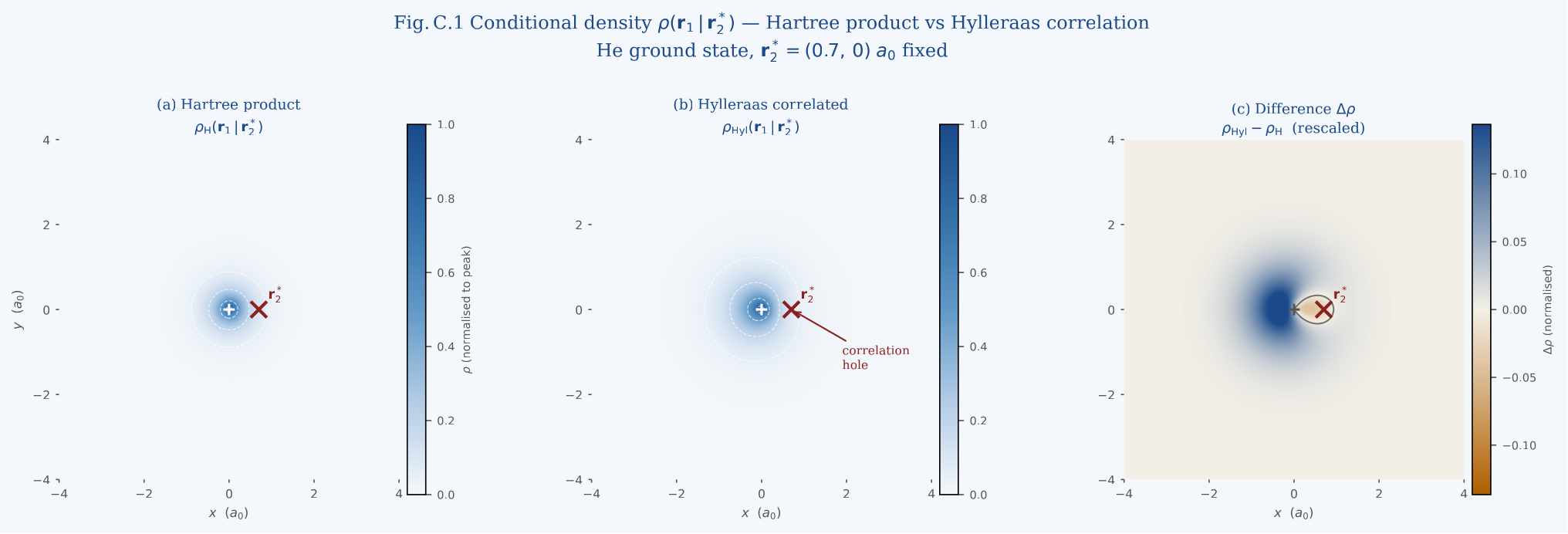
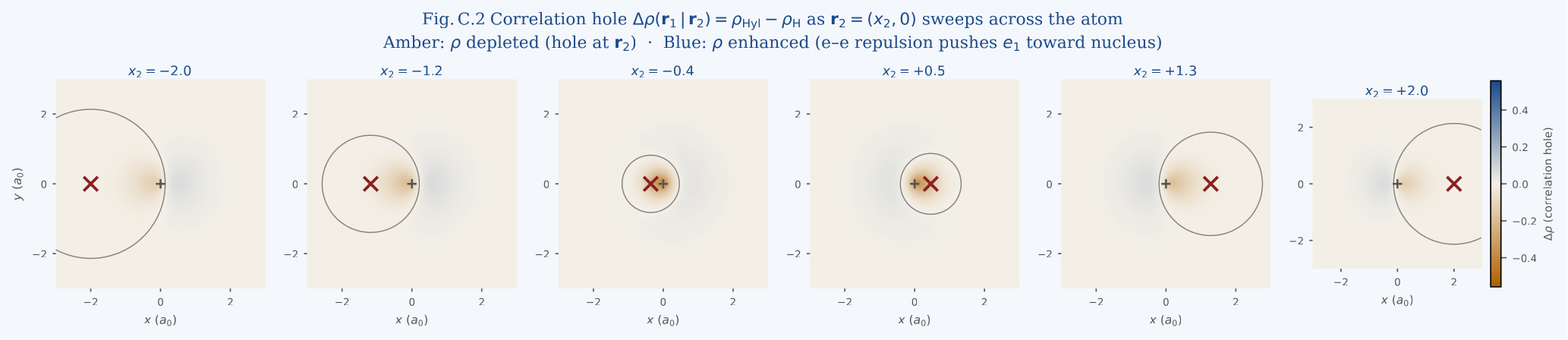
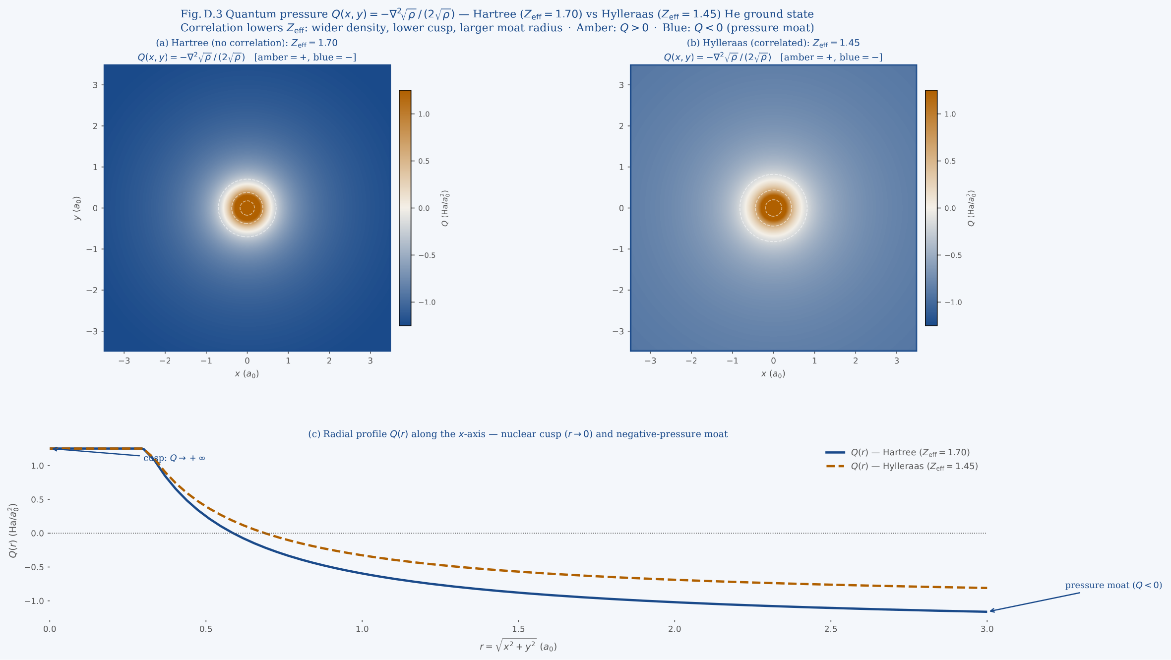
Figures 20–22 provide three complementary spatial views of how electron-electron correlation modifies the coherence field. Figure 20 shows the conditional density \(\rho(\mathbf{r}_1\,|\,\mathbf{r}_2^*)\) for a fixed reference position \(\mathbf{r}_2^*\): the Hylleraas result exhibits a clear dip (the correlation hole) absent in the Hartree product. Figure 21 extends this to a scan of \(\mathbf{r}_2^*\) positions, confirming that the hole follows the reference electron across the atom. Figure 22 complements these density-based views with the quantum pressure \(Q(x,y) = -\nabla^2\!\sqrt{\rho}/(2\sqrt{\rho})\), which encodes the kinetic cost of density curvature: the positive amber cusp near the nucleus and the negative blue moat at intermediate radius both shift with \(Z_\mathrm{eff}\) when correlation is included.
Part V —Excited States, Oscillator
Strengths, and Transitions
Excited-State Fixed Points
The \(1snl\) excited states of helium are fixed points with higher energy than the ground state. The CFT recurrence must produce a hierarchy of fixed points whose energies match the experimental term values. The exchange splitting between singlet and triplet series is the key qualitative test.
\(1s2s\) states
Para: \(1s2s\ {}^1S_0\); both electrons have \(\ell = 0\); density is spherically symmetric with two radial shells.
Ortho: \(1s2s\ {}^3S_1\); one electron in \(1s\), one in \(2s\); must have antisymmetric spatial part and \(M_S \in \{-1, 0, +1\}\).
Exchange splitting: \(J(1s,2s) \approx 0.796\,\mathrm{eV}\); in CFT this must arise from the \(\pi\)-phase difference between the singlet and triplet mode pairs.
The \({}^3S_1\) state is the most studied metastable state in atomic physics; its lifetime encodes magnetic-dipole matrix elements.
\(1s2p\) states and the \(2^3P\) fine structure
Para: \(1s2p\ {}^1P_1\); odd parity; principal dipole-allowed transition from ground state at \(58.4\,\mathrm{nm}\).
Ortho: \(1s2p\ {}^3P_{0,1,2}\); fine-structure triplet.
The \(2^3P_J\) splitting is the most precisely measured two-electron QED quantity; current theoretical uncertainty is \(\sim 10\,\mathrm{kHz}\).
In CFT: the \(2p\) fixed points carry angular momentum \(\ell = 1\) (winding number in the \(\theta\)-\(\phi\) sector); fine-structure splitting requires spin–orbit coupling between the mode’s angular and spin phases.
Doubly excited (autoionizing) states
When both electrons are excited (e.g. \(2s2p\), \(2p^2\)), the atom sits above the ionization threshold; these are resonances that decay via Auger autoionization.
Fano resonances: the doubly excited states interfere with the continuum, producing asymmetric line shapes. The Fano profile is characterised by \(q\) and \(\Gamma\).
The lowest doubly excited state \(2s^2\ {}^1S_e\) at \(57.8\,\mathrm{eV}\) (relative to ground state) has been measured by electron–impact and photoionization spectroscopy.
In CFT: doubly excited states are unstable fixed points (saddle points in the Lyapunov landscape); their decay rate \(\Gamma\) corresponds to the imaginary part of the fixed-point eigenvalue.
Oscillator strengths and transition rates
Oscillator strength \(f_{if}\): measures dipole transition probability; \(f_{if} = \tfrac{2m_e\omega}{3\hbar} |\langle f|\hat{\mathbf{r}}|i\rangle|^2\).
For the \(1s^2\ {}^1S_0 \to 1s2p\ {}^1P_1\) transition: \(f = 0.2762\); among the largest in the spectrum.
In CFT: \(f_{if}\) is the overlap integral between the initial and final fixed-point density profiles multiplied by the phase gradient coupling to the photon mode.
Part VI —Helium-3 vs. Helium-4 in
CFT
Nuclear Spin Statistics and the Isotope Effect
\({}^3\mathrm{He}\) (spin-\(\tfrac{1}{2}\), fermion) and \({}^4\mathrm{He}\) (spin-0, boson) differ in nuclear mass and nuclear spin. At the atomic level the electronic structure is almost identical; the differences are at the \(\sim\) ppm level (isotope shift). At the macroscopic level the difference is dramatic: \({}^4\mathrm{He}\) condenses into a superfluid at \(2.17\,\mathrm{K}\); \({}^3\mathrm{He}\) does not superfluid until \(\sim 2.5\,\mathrm{mK}\).
Electronic isotope shift
Normal mass shift: correction \(\propto m_e/M_\mathrm{nuc}\); shifts energy levels by \(\sim\) ppb relative.
Specific mass shift: two-body correction involving the mass-polarization operator \(\hat{T}_\mathrm{mp} = -(\mathbf{p}_1 \cdot \mathbf{p}_2)/M_\mathrm{nuc}\); unique to multi-electron atoms.
Field shift: nuclear charge distribution differs between \({}^3\mathrm{He}\) and \({}^4\mathrm{He}\); contributes a nuclear-size correction.
The \(2^3S_1 \to 2^3P_{J}\) transition isotope shift is \(\sim -600\,\mathrm{MHz}\); measured at kHz precision.
Nuclear spin effects
\({}^3\mathrm{He}\): nuclear spin \(I = \tfrac{1}{2}\) couples to electron spin and orbital angular momentum; hyperfine structure splits each electronic level into \(F = J \pm \tfrac{1}{2}\) components.
Hyperfine coupling constant \(a\): proportional to the electron density at the nucleus (\(s\)-states) and to the tensor interaction (\(p,d,\ldots\)-states).
In CFT: hyperfine coupling requires the phase field of the electron to be modulated by the nuclear spin mode; a nuclear-spin mode couples to the electronic fixed point.
\({}^4\mathrm{He}\): \(I = 0\); no hyperfine structure.
Can CFT distinguish bosonic and fermionic nuclei?
Statistics of the nucleus in CFT. The nucleus in single-atom CFT is treated as an external potential \(-Z/r\). Nuclear spin statistics affect:
The phase factor of the nuclear coherence field when two identical nuclei are exchanged (relevant for the He dimer and liquid phases).
The coupling between electronic and nuclear phase modes (hyperfine structure).
The symmetry class of the full wavefunction \(\Psi_\mathrm{nuc} \otimes \Psi_\mathrm{elec}\): for \({}^3\mathrm{He}\) (overall fermion), \(\Psi_\mathrm{elec}\) must have specific exchange symmetry given the nuclear spin state.
In CFT language: does the winding number of the nuclear phase field uniquely determine whether the nuclear mode is bosonic or fermionic? Does this induce the correct exchange symmetry on the electronic fixed point?
Part VII —Liquid Helium and Superfluid
Phases
Liquid \({}^4\mathrm{He}\): Bose Superfluid
Superfluid \({}^4\mathrm{He}\) is the paradigmatic macroscopic quantum system. Its order parameter is a complex field \(\Phi(\mathbf{r}, t)\) satisfying a nonlinear Schrödinger (Gross–Pitaevskii) equation — structurally identical to the CFT equation. This is not a coincidence: the superfluid order parameter is a coherence field fixed point.
Phase diagram and lambda transition
At atmospheric pressure: gas \(\to\) normal liquid (He I) at \(4.21\,\mathrm{K}\); He I \(\to\) superfluid (He II) at \(T_\lambda = 2.172\,\mathrm{K}\) (the lambda transition).
He II supports two-fluid behaviour: a superfluid component \(\rho_s(T)\) coexisting with a normal component \(\rho_n(T) = \rho - \rho_s\).
At \(T = 0\): \(\rho_s = \rho\) (all superfluid); but even at \(T = 0\), quantum depletion means only \(\sim 9\%\) of atoms are in the zero-momentum condensate (strong interactions).
The lambda transition is in the 3D XY universality class; critical exponent \(\nu \approx 0.6717\).
Gross–Pitaevskii equation as CFT
Gross–Pitaevskii / CFT identification. The superfluid order parameter \(\Phi(\mathbf{r}, t)\) satisfies \[\begin{equation}i\hbar\,\partial_t \Phi = \Bigl[-\tfrac{\hbar^2}{2m}\nabla^2 + V_\mathrm{ext}(\mathbf{r}) + g|\Phi|^2\Bigr]\Phi, \label{eq:gpe}\end{equation}\] with \(g = 4\pi\hbar^2 a_s/m\) and \(s\)-wave scattering length \(a_s = 2.9\,\mathrm{nm}\) for \({}^4\mathrm{He}\). This is precisely the CFT equation of motion \(\eqref{eq:cft_6d}\) in 3D, with the nonlinear coupling \(g\) set by the interatomic scattering length.
Key insight: the superfluid is a coherence fixed point at the macroscopic scale. The condensate wavefunction \(\Phi\) is a macroscopic fixed point of the many-body propagator.
Quantised vortices in CFT
Vortex solution: \(\Phi(\mathbf{r}) = f(r)e^{in\theta}\) with winding number \(n \in \mathbb{Z}\); core radius \(\xi = \hbar / \sqrt{2m g |\Phi|^2}\) (healing length).
For \({}^4\mathrm{He}\): \(\xi \approx 0.1\,\mathrm{nm}\); quantised circulation \(\kappa_n = nh/m\).
Vortex stability: \(n = 1\) is stable; \(n \ge 2\) unstable (decay into \(n\) unit vortices).
Feynman–Onsager quantisation: precursor to the fixed-point classification in the CFT catalog; superfluid vortex is a Class I fixed point.
Vortex lattice (Abrikosov analogue): in rotating He II, vortex lines arrange into a triangular lattice; Class IV fixed point.
Beyond Gross–Pitaevskii: strong coupling
GP equation is a mean-field (dilute-gas) approximation; liquid helium is strongly interacting (\(n a_s^3 \sim 0.2\)).
Beyond GP: Bogoliubov spectrum (phonons and rotons) requires the full many-body Hamiltonian.
The roton minimum at wavevector \(k_0 = 1.9\,\text{\AA}^{-1}\) is not captured by GP/CFT at mean-field level.
CFT route to roton: mode coupling between the condensate field and short-wavelength fluctuations; the BCH curvature correction as a source of non-linear dispersion.
Landau critical velocity \(v_c\): the minimum group velocity of elementary excitations; \(v_c \approx 60\,\mathrm{m/s}\).
Roton minimum in CFT. Can the coherence field, with a single nonlinear coupling \(g\), reproduce the phonon–roton spectrum of He II, including the roton minimum at \(\Delta_\mathrm{roton}/k_B = 8.65\,\mathrm{K}\)? Or does the roton require a multi-mode CFT with a separate “roton mode” fixed point?
Liquid \({}^3\mathrm{He}\): Fermionic Superfluid
Superfluid \({}^3\mathrm{He}\) is a fermionic superfluid in which pairs of atoms condense in a \(p\)-wave (\(\ell = 1\)) state, forming an anisotropic order parameter. It is the condensed-matter analogue of a triplet superconductor. Describing it in CFT requires a pair-field (Gorkov) formulation.
Cooper pairing and the order parameter
Superfluidity in \({}^3\mathrm{He}\): BCS-like Cooper pairs with \(\ell = 1\), \(S = 1\) (spin-triplet, \(p\)-wave).
Transition temperature: \(T_c \approx 2.5\,\mathrm{mK}\) (\(\approx 10^{-3}\) of \(T_\lambda\) for \({}^4\mathrm{He}\)).
Order parameter: a \(3 \times 3\) matrix \(A_{\mu i}(\mathbf{r})\) (spin \(\times\) orbital); the condensate is described by a tensor field, not a scalar.
Superfluid phases:
He-3-A phase: axially symmetric, non-unitary; characterized by an \(\hat{\ell}\)-texture (orbital anisotropy field).
He-3-B phase: isotropic gap; most stable at low pressure; time-reversal invariant.
CFT description of fermionic condensate
Gorkov/BdG CFT: replace the single complex field \(\Phi\) with a Nambu spinor \((\psi_\uparrow, \psi_\downarrow^\dagger)\); the pair amplitude \(\Delta(\mathbf{r}, \mathbf{r}') = \langle \psi_\uparrow (\mathbf{r})\psi_\downarrow(\mathbf{r}')\rangle\) is the order parameter.
Fixed point of the BdG propagator: the gap equation as a self-consistency condition on the phase field of \(\Delta(\mathbf{r})\).
For \(p\)-wave pairing: the fixed point must carry orbital angular momentum \(\ell = 1\); this is a winding-number-1 fixed point in the orbital sector.
Topological superfluids: He-3-B is a topological superfluid with a \(\mathbb{Z}_2\) invariant; the boundary hosts Majorana surface modes. Can CFT classify these topological fixed points?
Tensor order parameter in CFT. CFT is currently formulated with a scalar complex field. The \(p\)-wave order parameter of He-3 is a tensor. Does the tensor structure emerge from a product of winding-number-1 scalar fields, or does CFT require a genuine tensor extension? How do topological invariants (Pontryagin index, \(\mathbb{Z}_2\) classification) arise in the scalar-CFT language?
Defects and textures in He-3
The \(\hat{\ell}\)-texture in He-3-A: spatial variation of the orbital anisotropy axis; supports half-integer vortices.
Mermin–Ho relation: \(\nabla \times \mathbf{v}_s = (\hbar/4m) \hat{\ell} \cdot (\nabla\hat{\ell} \times \nabla\hat{\ell})\); relates orbital texture to superfluid circulation.
Skyrmion textures: topologically stable configurations of \(\hat{\ell}\); each skyrmion carries a Pontryagin number \(\mathcal{Q} \in \mathbb{Z}\).
In CFT: skyrmions are fixed points of the tensor field analogous to vortex fixed points in the scalar case.
Part VIII —Unsolved Problems and the CFT
Research Agenda
Precision Tests and Unresolved Discrepancies
Despite helium being the best-studied multi-electron atom, several precision measurements disagree with theory at the level of \(1\)–\(100\,\mathrm{kHz}\), and the doubly-excited resonance spectrum is incompletely characterised. CFT may offer new computational approaches to these hard problems.
The \(2^3P\) fine-structure discrepancy
The \(\nu_{01} \equiv 2^3P_1 - 2^3P_0\) splitting: measured to \(\delta\nu \sim 150\,\mathrm{Hz}\) precision; theory (Drake, Pachucki) has an uncertainty of \(\sim 10\,\mathrm {kHz}\) from uncalculated higher-order QED terms.
Current status (2024): experiment and theory agree to \(\sim 1\,\mathrm{kHz}\); residual discrepancy \(\sim 0.3\, \sigma\) could be statistical.
CFT angle: the spin–orbit splitting is sensitive to the phase structure of the fixed point near the nucleus; can the BCH curvature correction contribute a calculable, non-trivial correction to the fine-structure interval?
Near-threshold double photoionization
Above the double ionization threshold (\(79.0\,\mathrm{eV}\)), both electrons are liberated; the joint angular/energy distribution is described by the Wannier exponent.
Wannier threshold law: the total cross section near threshold scales as \(\sigma(E) \propto (E - E_\mathrm{thr})^{1.127}\); confirmed experimentally but the coefficient is not accurately known.
In CFT: double ionization is the decay of the two-electron fixed point into two continuum modes; the threshold exponent may be derivable from the instability spectrum of the fixed point.
Doubly excited resonances (Fano resonances)
Complete classification of \(2\ell 2\ell'\) resonances: positions \(E_r\) and widths \(\Gamma\) are measured, but ab initio calculations beyond the \(K\)-matrix method remain challenging.
Propensity rules: certain \(\Delta n\) transitions have anomalously small Auger rates; explained by symmetry in hyperspherical coordinates.
CFT approach: doubly excited states as saddle-point fixed points in 6D; the Fano profile width \(\Gamma\) as the fixed-point instability eigenvalue.
The helium dimer (\(\mathrm{He}_2\))
The helium dimer is bound by the van der Waals potential with a well depth of only \(\sim 11\,\mu\mathrm{Ha}\) (\(\sim 0.94\,\mathrm{mK}\)); one of the most weakly bound diatomics.
The bond length \(\sim 52\,a_0\) is unusually large; the ground vibrational state has a probability density extending to \(\sim 200\,a_0\).
In CFT: the dimer is a two-centre fixed point; the tunnelling mode between the two atoms generates the tiny binding energy.
Efimov states: three-body \(\mathrm{He}_3\) trimers just below the dimer–atom threshold; geometric tower of bound states with ratio \(\sim 22.7\) between successive binding energies.
CFT and Efimov: are Efimov states a tower of fixed points related by a discrete scaling symmetry?
CFT Research Programme for Helium
The following problems are ordered from most immediately tractable (using existing CFT numerical machinery) to most speculative (requiring theoretical extensions).
Tier 1: Extensions of existing CFT tools
Two-fluid SCF: extend the existing 1D/2D CFT propagator to a self-consistent two-field iteration; verify convergence to the Hartree–Fock energy \(-2.861\,680\,\,\mathrm{Ha}\).
Exchange splitting: implement the \(\pi\)-phase constraint for the triplet state; demonstrate that the singlet–triplet energy difference reproduces the exchange integral \(J(1s,2s)\).
Radial density profile: compare the self-consistent CFT density \(\rho^*(r)\) to the Hylleraas result and to MP2/CCSD benchmark.
Mode spectrum: compute the Bogoliubov spectrum of the SCF fixed point; identify the first few excitation energies; compare to \(1s2s\) and \(1s2p\) levels.
Tier 2: New theoretical developments
Pair-density CFT: formulate the energy functional in terms of \(\Gamma(\mathbf{r}_1, \mathbf{r}_2)\); derive the correlation energy as a phase-gradient coupling term.
BCH curvature and relativistic corrections: show that the BCH correction to the two-mode product propagator generates the mass–velocity and Darwin terms at order \(\alpha^2\).
Fano resonances as unstable fixed points: apply complex-eigenvalue analysis to the 6D CFT propagator near a doubly-excited state; extract \(E_r\) and \(\Gamma\).
Liquid-helium CFT: formulate the GP equation as the \(T = 0\) CFT for \({}^4\mathrm{He}\); derive the phonon–roton spectrum from multi-mode CFT; compare to neutron-scattering data.
Tier 3: Speculative / foundational questions
Tensor CFT for He-3: extend the scalar coherence field to a spinor or tensor order parameter; classify the A and B phases as fixed points of the extended theory.
Topological fixed points: can the \(\mathbb{Z}_2\) invariant of He-3-B be computed from the CFT winding-number structure?
Fermi statistics from phase winding: derive the Pauli exclusion principle as a topological obstruction in the two-particle phase field.
Nuclear coherence: the nucleus as a coherence field fixed point; nuclear recoil and finite-size corrections as phase shifts of the nuclear mode; unified atomic + nuclear CFT.
Lambda transition in CFT: is the 3D XY critical point a marginal fixed point of the CFT in the renormalisation-group sense? Can the critical exponent \(\nu \approx 0.6717\) be derived from CFT mode-coupling?
Part IX —Computational Strategy and
Outlook
Numerical Methods for Two-Electron CFT
Grid strategies
1D radial CFT (SCF): use existing propagator with \(L \sim 20\), \(N_\mathrm{steps} \sim 300\); two fields iterated to self-consistency; cost \(\mathcal{O}(N^1)\).
3D CFT on a radial grid with spherical harmonic decomposition: \(\psi(\mathbf{r}, t) = \sum_{\ell m} \psi_{\ell m}(r, t) Y_\ell^m(\hat{r})\); cost \(\mathcal{O}(N_r \cdot \ell_\mathrm {max}^2)\).
6D CFT: full two-electron grid; practical only for \(N_r \lesssim 30\) per electron per dimension; Hylleraas coordinates preferred.
Convergence criteria
Fixed-point convergence: \(\|\psi^{(n+1)} - e^{i\alpha} \psi^{(n)}\|_2 < \epsilon\); use \(\epsilon \sim 10^{-8}\) for energy to \(\mu\,\mathrm{Ha}\) accuracy.
Energy convergence: monitor \(\langle \hat{H}\rangle / N_\mathrm {modes}\) per SCF iteration; compare to published HF/CI benchmarks.
Density convergence: \(\|\rho^{(n+1)} - \rho^{(n)}\|_1 < \epsilon_\rho\); key for pair-density formulation.
Benchmarking protocol
Proposed benchmarking ladder for CFT–helium.
Reproduce \(E_\mathrm{He}^+\) (one electron) to machine precision: validates 3D single-particle CFT with \(Z = 2\).
Reproduce \(E_\mathrm{HF}\) to \(0.01\,\mathrm{mHa}\): validates SCF iteration.
Reproduce exchange splitting \(J(1s,2s)\) to \(0.01\,\mathrm{eV}\): validates antisymmetry implementation.
Reproduce \(E_\mathrm{corr}\) to \(1\,\mathrm{mHa}\): validates beyond-mean-field phase coupling.
Reproduce \(2^3P_J\) fine-structure interval to \(1\,\mathrm{MHz}\): validates relativistic/BCH correction.
Outlook
Helium is the Drosophila of quantum chemistry; a CFT that passes the benchmarking ladder in Sec. 14 establishes it as a quantitative tool for multi-electron atoms.
The natural next step after helium is lithium (\(Z = 3\), three electrons) and then the helium isoelectronic series (\(Z = 3,\ldots,10\)); the scaling of fixed-point properties with \(Z\) is a stringent test.
For liquid helium, the CFT/GP identification is exact at the mean-field level; the research frontier is whether CFT can go beyond GP to capture strong correlations (\(n a_s^3 \gtrsim 0.1\)) and the roton without introducing an empirical dispersion relation.
The fermionic case (He-3 superfluidity, topological phases) is the deepest theoretical challenge: it requires a tensor or multi-component coherence field, or a derivation of fermionic statistics from bosonic phase topology.
Precision atomic physics (fine-structure, isotope shifts, QED Lamb shifts) offers the highest-resolution tests; agreement at the \(10\,\mathrm{kHz}\) level would be a remarkable vindication of CFT as a fundamental theory.
Key Constants and Atomic Units
| Quantity | Symbol | Value (SI) |
|---|---|---|
| Bohr radius | \(a_0\) | \(5.2918 \times 10^{-11}\,\mathrm{m}\) |
| Hartree energy | \(E_h\) | \(4.3598 \times 10^{-18}\,\mathrm{J} = 27.211\,\mathrm{eV}\) |
| Fine-structure constant | \(\alpha\) | \(7.2974 \times 10^{-3}\) |
| Electron mass | \(m_e\) | \(9.1094 \times 10^{-31}\,\mathrm{kg}\) |
| \({}^4\mathrm{He}\) nuclear mass | \(M_4\) | \(6.6465 \times 10^{-27}\,\mathrm{kg}\) |
| \({}^3\mathrm{He}\) nuclear mass | \(M_3\) | \(5.0082 \times 10^{-27}\,\mathrm{kg}\) |
| \({}^4\mathrm{He}\) scattering length | \(a_s\) | \(2.9\,\mathrm{nm}\) |
| He-II \(\lambda\)-point | \(T_\lambda\) | \(2.172\,\mathrm{K}\) |
| He-3-B \(T_c\) | \(T_c\) | \(\approx 1.1\,\mathrm{mK}\) (at melting pressure) |
CFT Equation Reference
For convenient reference, the central equations of CFT as used in this outline:
Single-particle propagator: \[U(\delta t) = e^{-i\hat{H}\delta t/\hbar}, \qquad \hat{H} = -\tfrac{\hbar^2}{2m}\nabla^2 + V(\mathbf{r}) + g|\psi|^2. \tag{CFT-1}\]
Fixed-point condition: \[U(\delta t)\,\psi^{*}_{} = e^{i\alpha}\psi^{*}_{}, \qquad \alpha = -E\delta t/\hbar. \tag{CFT-2}\]
Two-electron propagator (configuration space): \[i\hbar\,\partial_t \Psi(\mathbf{r}_1,\mathbf{r}_2,t) = \Bigl[\hat{H}_1 + \hat{H}_2 + \tfrac{1}{r_{12}} + g|\Psi|^2\Bigr]\Psi. \tag{CFT-3}\]
Gross–Pitaevskii / superfluid CFT: \[i\hbar\,\partial_t \Phi(\mathbf{r},t) = \Bigl[-\tfrac{\hbar^2}{2m}\nabla^2 + V_\mathrm{ext} + \tfrac{4\pi\hbar^2 a_s}{m}|\Phi|^2\Bigr]\Phi. \tag{CFT-4}\]
Bogoliubov–de Gennes (fermionic case): \[\begin{pmatrix} H_0 - \mu & \Delta(\mathbf{r})\\ \Delta^*(\mathbf{r}) & -(H_0 - \mu) \end{pmatrix} \begin{pmatrix}u_n\\v_n\end{pmatrix} = E_n\begin{pmatrix}u_n\\v_n\end{pmatrix}. \tag{CFT-5}\]
Driver
analysis/helium_breit_partition.py, validated against published He \(1\,{}^1S\) benchmarks before assembly: \(\langle\delta^3(r_1)\rangle = 1.809\) (ref. \(1.810\)), \(\langle\delta^3(r_{12})\rangle = 0.108\) (ref. \(0.106\)), \(\langle\sum_i p_i^2\rangle = 5.807 = -2E_0\) (virial), and \(\langle\sum_i p_i^4\rangle = 102.9\) (ref. \(108.2\); the residual is the slow cusp convergence of \(p^4\) in a \(10\)-term basis).↩︎Computed by
analysis/helium_cft.py; here a \(10\)-term basis at \(\zeta = 1.807\) gives \(E_0 = -2.9035\,\,\mathrm{Ha}\), within \(0.18\,\mathrm{mHa}\) of the Pekeris benchmark.↩︎